Page 223 - Special Topic Session (STS) - Volume 1

STS425 Zaitul Marlizawati Z. et al.
i 
s
P  b x  y  0 i I , j  J
i
, i j
j
j J (10)
Equation (9) refers to the limitation plant capacity for crude distillation unit
(CDU) and catalytic cracker unit. Meanwhile equation (10) refers to mass
balances constraints classified as fixed production yields, fixed blends and
unrestricted balances.



x  z  z  d ,i I random  , I s
S
i , i s , i s , i s demand (11)

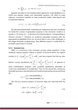
The demand deterministic constraints are replaced by the new constraints
to model the number of generated scenarios in the stochastic model as in
equation (11) where d , i s is demand of finished products corresponding to

demand scenario s . However, to construct reasonable scenarios with the
appropriate probabilities from the historical data is one of the challenges in
two-stage stochastic programming. Thus effective scenario construction for
stochastic parameters is needed.

2.2.2 Scenario tree
GBM is a continuous time stochastic process where logarithm of the
randomly varying quantity follows a random movement where the explicit
   2 
solution is S  S exp    t    W and has property that the log ratio
t 
0
t
 2   
 S     2  
follows normal distribution, ln  t  ~ N    , t   2 t   . In general to
 S  t 1  2   
solve mathematical program with uncertain parameters described as
continuous distributions is complicated. Thus we discretized the continuous
stochastic process in discrete binomial model as proposed by Jarrow and Rudd
(9)
 S u with probability p
S t 1   t
 S d with probability 1- p (12)
t
The first and second moment of binomial steps are matching with the
GBM.
   2
p lnu  (1 p )ln d      t 
 2  (13)

p (1 p  ) lnu  ln  d 2   2 t 

212 | I S I W S C 2 0 1 9