Page 298 - Special Topic Session (STS) - Volume 1

STS430 Eustasio D.B. et al.
1 ⁄
2
1
2
( , … , ) = { ∑ ( , )} .

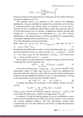
1

2
2

=1
Empirical versions of the barycenter are analyzed in [8, 25]. Similar ideas have
also been developed in [6, 15].
This quantity, which is an extension of the variance for probability
distributions is a good candidate to evaluate the concentration of a collection
of measures around their Fréchet mean. In particular, it can be used to
measure the fit to a distribution deformation model. More precisely, assume
as in the Introduction that we observe J independent random samples with
sample {1, … , } consisting of iid observations , … , , with common
1,
distribution . We assume that is a family (parametric or nonparametric)

of invertible warping functions and denote = × ⋯ × .
1

Then, the deformation model assumes that
there exists ( , … ) ∈ and iid ( ) 1≤≤,1≤≤ such that for all ∈
∗
∗
,

1
−1
∗
{1, … , }, , = ( ) (ℰ ). (1)
,

∗
∗
Equivalently, the deformation model (1) means that there exists ( , … , )
1

such that collection of ( ) taken over all ∈ {1, … , } and {1, … , } is iid
∗
,

or, if we write ( ) for the distribution of ( ) , that there exists

,

∗
∗
( , … , ) such that ( ) = ⋯ = ( ) .
∗
∗
1

1
1
We propose to use the Wasserstein variation to measure the fit of model
(1) through the minimal alignment cost

() = { ( ), … , ( )} . (2)
1

1

( 1 ,…, )∈

Let us assume that ( ), … , ( ), ( , … , ) ∈ are in (ℝ ). If the
1

1

1

deformation model (1) holds, then () = 0 . Under the additional mild

assumption that the minimum in (2) is attained, we have that the deformation
model can be equivalently formulated as () = 0 and a goodness-of-fit test

to the deformation model becomes, formally, a test of
ℋ ∶ () = 0 vs. ℋ ∶ () > 0. (3)
0

A testing procedure can be based on the empirical version of (),

namely,

, () = { ,1 ( ), … , ( )} , (4)

1
( 1 ,…, )∈
where , ( ) denotes the empirical measure on ( ), … , ( ). We

,

1,
would reject the deformation model (1) for large values of , ().
As noted in [16, 26], the testing problem (3) can be considered as a mere
sanity check for the deformation model, since lack of rejection of the null does
not provide statistical evidence that the deformation model holds.
Consequently, as in the cited references, we will also consider the alternative
testing problem
287 | I S I W S C 2 0 1 9