Page 15 - Special Topic Session (STS) - Volume 4

STS556 Mohd Bakri A. et al.
of smoothing is done by simulation of signal and noise. The process of
simulation is based on procedure from Conradie et al., 2009. Generally, data
can be decomposed into the following components:

Datat = Signalt + Noiset = Xt (12)

The signal is a combination of sinusoidal function with linear curve:


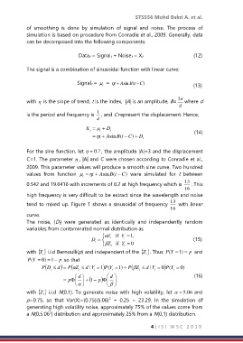
Signalt =  = t + A sin B (t − C ) (13)
t

with  is the slope of trend, t is the index, |A| is an amplitude, B=  2 where d
d
is the period and frequency is 1 , and C represent the displacement. Hence,
d

X =  t + D t (14)
t
= t + Asin B( t − ) D t
C +


For the sine function, let = 7 . 0 , the amplitude |A|=3 and the displacement
C=1. The parameter  , |A| and C were chosen according to Conradie et al.,
2009. This parameter values will produce a smooth sine curve. Two hundred
values from function  = t + A sinB (t − C ) were simulated for t between
t
0.542 and 19.6416 with increments of 0.2 at high frequency which is 13 . This
16
high frequency is very difficult to be extract since the wavelength and noise
tend to mixed up. Figure 1 shows a sinusoidal of frequency 13 with linear
16
curve.
The noise, {Dt} were generated as identically and independently random
variables from contaminated normal distribution as
 Z if Y = ,1
D =  t t (15)
t
  Z t if Y t = 0
with   i.i.d Bernoulli(p) and independent of the  . Thus P( Y = ) 1 = p and
Z
Y
t
t
P( Y = ) 0 = 1 − p so that
P (D  d ) = P (Z  d |Y = 1 ) (YP = ) 1 + P (Z  d |Y = 0 ) (YP = ) 0
t t t t t t t
 d   d  (16)

= p    + (1− p )    . 
     
with   i.i.d N(0,1). To generate noise with high volatility, let  = . 5 06 and
Z
t
p=0.75, so that Var(X)=(0.75)(5.06) + 0.25 = 23.29. In the simulation of
2
generating high volatility noise, approximately 75% of the values come from
2
a N(0,5.06 ) distribution and approximately 25% from a N(0,1) distribution.
4 | I S I W S C 2 0 1 9