Page 350 - Invited Paper Session (IPS) - Volume 2

IPS273 Charlotte L. et al.
The obtained equation can be equivalently seen as a rank-one matrix
factorization of the Gibbs kernel −M/ that depicts the joint interactions
between two sets of objects underlying α and β. On the other hand, in the
extreme case when λ → ∞, the Gibbs kernel −M/ becomes a matrix of ones
leading to a degenerate solution where u and v are vectors of ones.
Finally, we note that when λ does not tend to infinity, one may retrieve
a particular type of tri-factor factorization from the solution of the
regularized OT problem. To see that, we can rewrite the factorization of the
optimal coupling matrix as follows:

1 1
⋆
−M/ = diag ( ) (, )diag ( ),

where vectors u, v and the optimal coupling matrix (, ) are
⋆

unknown. This formulation is reminiscent of a popular co-clustering
method called Tri-NMF (Ding et al, 2008) formulated as the following
optimization problem over ∈ ℝ × , ∈ ℝ × , ∈ ℝ × for some ∈
+
+
+
ℝ × :
+

≃ , = , = ,

where W and H are low-rank approximations of features and instances,
respectively, S is a matrix of associations between them and the
orthogonality constraints are added to ensure the uniqueness of the
factorization and the ease of interpretability for clustering. From this
formulation, we note that co-clustering solutions provided by u and v can
be seen as full-rank approximations of matrices W and H while the
⋆
meaning behind (, )remains similar to that of S. Furthermore,

1
1
matrices diag ( ) and diag ( ) corresponding to W and H naturally fulfill

the orthogonality constraints up to a scaling factor. This point of view tells
us that regularized optimal transport can be equivalently seen as both
rank-one and full-rank matrix factorizations of the Gibbs kernel −M/
where in both cases the latent low-rank structure for rows and columns
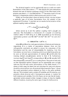
should be extracted from one-dimensional objects u and v. Figure 1 shows
the cluster-generated vectors obtained by them on the same synthetic
data set. The simulated matrix contains 60 variables and 60 instances, and
presents a block structure with 3 homogeneous groups, or clusters, for
both instances and variables. From this figure, we can see that all cluster-
generated vectors present similar changes in slope, at close but slightly
different locations, revealing the same type of steps for both u and v.

337 | I S I W S C 2 0 1 9