Page 38 - Special Topic Session (STS) - Volume 1

STS346 Abu Sayed M. et al.
1
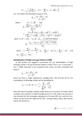
ˆ      (x i  X ˆ i ) 2   (y i  ˆ   X ˆ ˆ i ) 2 
2
n  2
and we obtain the estimated values of X as

ˆ
X i   x i ˆ (  y i  ) ˆ 
(   )
ˆ 2
y  ˆ   ˆ x and
where
  X ˆ y  ˆ   X 
ˆ
ˆ
  i i i
 X i 2
ˆ
ˆ
ˆ
ˆ
(   2 )( S xy  S yy  n 3 x 2  n  ˆ x 2 )

ˆ
ˆ
 2  y i 2  2  ˆ S xy   2 S yy  n 4 x 2  2n  ˆ 2 x 2
ˆ
gives S   ( S  S )  S  0 and that implies
ˆ 2
xy xx yy xy
S ) 
2
S (   S (   S )  4 S 2
ˆ
  yy xx yy xx xy
S 2 xy
 y  x
where, y  i , x  i ,S   y 2  yn 2 ,S   x 2  xn 2 and
n n yy i xx i
S xy   x i y i  xn y

Identification of High Leverage Points in LFRM
In this section we suggest a procedure for the identification of high
leverage points in linear functional relation model. From a set of observed x
and y (both assumed to be measured with error), we have estimated the
fixed-X
ˆ
X   x i ˆ (  y i  ) ˆ 
i
(   )
ˆ 2
Since we have a single explanatory variable here, the formula (5) for the

computation of leverage values can be simplified as

2
ˆ
ˆ
ˆ
T
w ˆ  x ( X T X)  1 x ˆ = 1  X ˆ i  X ˆ
ii
i
i
n n  2
 X ˆ i  X ˆ
 i 1
Since the above formula contains mean and sum of squares of means which
could be very sensitive to high leverage points. For this reason we propose a
new formula for the leverages analogous to formula (20), but here the non-
robust components are replaced by their corresponding robust alternatives.
Hence the formula is

27 | I S I W S C 2 0 1 9