Page 36 - Special Topic Session (STS) - Volume 1

STS346 Abu Sayed M. et al.
between a LRM and a LFRM is that in LRM it is assumed that the explanatory
variable is free from error but in LFRM it is subjected to error.

2. Methodology
In regression analysis it is sometimes very important to know whether any
set of X-values are exerting too much influence on the fitting of the model.
According to Hocking and Pendleton (1983) "high leverage points are those
for which the input vector x , in some sense, far from the rest of the data." Let
i
us consider a k variable regression model

Y  X   (3)
A set of influential X-values is known as a high leverage point. The OLS residual
vector can be expressed in terms of the true disturbance vector as
ˆ
 ˆ = Y  Y = (I  )W  (4)
where the matrix W  X( X T X) 1  X given in (4) is generally known as weight
T
matrix or leverage matrix. The weight matrix W reflects joint effect of k
regressors on the fitted responses. Writing the data matrix of k explanatory
T
variables as X  x , x , x , n  , the i-th diagonal element of the weight matrix
1
2
T
W is defined as w  x ( X T X)  1 x (5)
i
i
ii
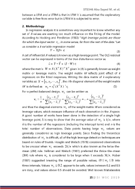
For a perfect balanced design, w can be written as
ii
1 x  x  2 x  x  2 x ip  x .p  2
w   1 i 1 .  2 i 2 . ... 
i  2  2  2
n  x 1 i  x 1 .  x 2 i  x 2 .  x ip  x .p
and thus the diagonal elements w of the weight matrix W are considered as
ii
leverage values, which measure influence of each observation in the X-space.
A good number of works have been done in the detection of a single high
leverage point. It is easy to show that the average value of w is nk , where
ii
k is the number of the regressors (including the intercept term) and n is the
total number of observations. Data points having large w values are
ii
generally considered as high leverage points. Since finding the theoretical
distribution of w is difficult, all of the high leverage detection techniques are
ii
based on rules of thumb. Hoaglin and Welsch (1978) considered observations
to be unusual when w exceeds k2 n which is also known as the twice-the-
ii
mean (2M) rule. Vellman and Welsch (1981) preferred the thrice-the–mean

(3M) rule where w is considered to be large when it exceeds k3 n. Huber
ii
(1981) suggested breaking the range of possible values, 0(  w ii  ) 1 into
three intervals. Values w ii  2 . 0 appear to be safe, values between 0.2 and 0.5
are risky, and values above 0.5 should be avoided. Well known Mahalanobis

25 | I S I W S C 2 0 1 9