Page 45 - Special Topic Session (STS) - Volume 1

STS353 H. Zhao et al.
exp{− exp()}, an extreme value distribution, while one can obtain the
proportional odds model by letting () = {1 + exp(−)} , the standard
−1
logistic distribution. Let denote the distribution function of given
. Then it is easy to see that model (1) can be equivalently expressed as

(1 − ()) = () − , where −1 () = 1 − ().

0
0
In the following, for inference about model (1), it will be assumed that
one only observes clustered interval-censored data given by { =

( , , ; = 1, … , ); = 1, … , } where ( , ] denotes the observed

interval for as < ≤ . Also we will assume that the cluster sizes

may contain some relevant information about or is informative, but given

, and are independent of or we have independent interval

censoring (Sun, 2006; Zhang et al., 2005). In other words, we have
( ≤ | = , = , < ≤ , ) = ( ≤ | < ≤ )

,
with respect to censoring intervals ( , ]′. Furthermore we will assume

that the failure times of interest ’s may be related to the cluster sizes ′.

Before presenting the proposed WCR estimation procedure, we will first
briefly consider univariate interval-censored data or the situation where =

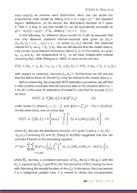
1 for all In this case, for estimation of model (1), note that for any pair ( )
,
we have
{( ≥ )| , } = ( ) (2)

∞
under mode (1), where = − and () = ∫ {1 − ( + )} ().

−∞
On the other hand, one can show that

{( ≥ )| , } = E {( ) −1 ∫ ∫ ( ≥ ) ( )| , }, (3)

where denotes the distribution function of given and = ( ) −

( ). Combining (2) and (3), Zhang et al.(2005) suggested that one can

estimate β based on the estimating equation
1
′

(1) () = ∑ ∑ ( ) { ̂ ̂ ∫ ∫ ( ≥ ) ̂ () ̂ () − ( )}

=1 =1
= 0, (4)
̂
where denotes a consistent estimator of , the ̂ ′ the ′ with the

̂
′ replaced by ′ and ∅′() the first derivative of ∅() having the form

′
with f denoting the density function of the . In the above, Since we assume

Z is a categorical variable here, it is natural to obtain the nonparametric
34 | I S I W S C 2 0 1 9