Page 206 - Contributed Paper Session (CPS) - Volume 1

CPS1280 Willard Z. et al.
In this paper, an analysis of winter rainfall variability for a selected region
in Western Cape, for the period 1980 to 2017 is presented. This is done by
firstly using Mann-Kendall Test (MK) to do a monthly analysis of winter rainfall
trend for the months May to August. Secondly, calculating the coefficient of
variability based on these months and then use kriging to find the spatial
spread of the rainfall variability.

2. Methodology
2.1 Mann-Kendell and Coefficient of Variation
Mann-Kendell trend Test (MK) is used to find any trend in the rainfall for
the given period. The advantage of MK is that it does not have any underlying
assumptions about the distribution of the data except that it must be
independent and identically distributed. It can indicate the temporal patterns
in a time series (Kendall, 1980). A correlation coefficient, where −1 ≤ ≤ 1 ,
denotes relative strength of the trend of the time series is computed. The
probability of this trend occurring by chance is also estimated, from which a
measure of statistical significance can be assigned.
A 5% level of significance is used such that if the probability estimate was
less than 0.05, the trend was deemed to be significant. The trend estimates
were calculated for the months May to August for all the 11 stations.
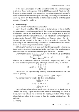
Given the time series , , , … , then the MK statistic, S, is defined as:
2,
1
3

−1
= ∑ ∑ sgn ( − ) (1)

=1 =1+1
where j and i are the data values in years and , respectively, with >,n is
the total number of years and sgn() is the sign function. Let j – i = then
1 > 0
sgn() = { 0 = 0 (2)
−1 < 0
The statistics S is approximately normally distributed, with mean zero and
variance given by:
() = ( − 1)(2 + 5)/18.
The standard normal variable Z is then formulated as
−1
> 0
√()
= 0 = 0 (3)
+1
< 0
{ √()
The coefficient of variation (CV%) is then calculated. CV%, also known as
“relative variability”, equals the standard deviation divided by the mean. It
measures how a value is varied around the mean (Label et al., 1987). Kriging
interpolation method is then used to find the spatial distribution of the
variation.
2.2 Kriging

195 | I S I W S C 2 0 1 9