Page 200 - Contributed Paper Session (CPS) - Volume 2

CPS1823 Ishapathik D. et al.
estimation of the unknown parameters and and the Gaussian copula
parameter in the above model.
3.1 Parameter Estimation
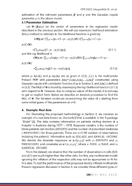
Let =[,,] be the vector of parameters in the regression model
described in the previous section. We will use maximum likelihood estimation
(MLE) method to estimate Θ. The likelihood function is given by
(|,)=∏:= [1 +(1−1 −2)()]×∏:= [2 +(1−1 –
2)()]

×∏:∉{,} [(1−1 −2)()], (3.1.1)
and the log-likelihood is
(|,)=∑:= log[1 +(1−1 −2)()]+∑:= log[2 +(1−1 –

2)()]
+∑:∉{,} log[(1−1 −2)()], (3.1.2)

where 1 ≡1() and 2 ≡2() are as given in (3.5), (⋅) is the multivariate
Poisson PMF with parameters ()=[1(),2(),…,()]′ constructed using
Gaussian copula with correlation function as in Section 3, and () is defined
in (3.3). The MLE of is found by maximizing the log-likelihood function (3.1.2)
with respect to . However, due to complex nature of the model, it is not easy
to get an explicit form. Below we describe an iterative procedure to find the
MLE of . The iteration continues incrementing the value of starting from
some initial guess of the parameters at =0.

4. Example: Real data
For illustrating the proposed methodology in Section 3, we consider an
example of a real data known as DoctorAUS that is available in the R-package
“Ecdat" [2]. The data contains information on patients visiting doctors at a
hospital in Australia during 1977 – 1978. Response variable is the number of
times patients visit doctors () and the number of prescribed medicines
( ) for those patients. There are =5190 number of observations
including the patients’ information such as ,, and .
We denote the bivariate responses as =[1,2]′ with 1 ≡ and 2
≡, and covariates as =[1,2,3]′, where 1 ≡, 2 ≡, and 3
≡ .
From the dataset, we observe that the number of observations in cells (0,0)
and (0,1) are much higher than the other cells. For this, any multivariate model
ignoring the inflation of the respective cells may not be appropriate to fit for
this data. To test the performance of the proposed doubly inflated multivariate
Poisson regression discussed in Section 3, we consider three different types of

189 | I S I W S C 2 0 1 9