Page 223 - Contributed Paper Session (CPS) - Volume 3

CPS1999 Pranesh K. et al.
years old. The main purpose of the application in this study is to model and
predict the effect of ocean heat content, (10 ^22 Joules) on the global sea ice
2
extent, (in million km ).

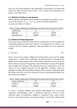
3.1. Method of Ordinary Least Squares
Fitted ordinary least squares (OLS) model to the global sea ice extent, and
ocean heat content, is y = + , where the fitted coefficients
1
0
and are shown in Table 2.
0
1

Table 2: Crisp Coefficients of Global Sea Ice Extent and Ocean Heat Content
Coefficients
1
0
Estimate 23.5114 -0.0614
Standard error 0.8360 0.0370

3.2. Method of Fuzzy Regression
This section aims to determine the best fuzzy regression model to explain the
relationship between ocean heat content, and global sea ice extent, and
compare with the classical regression. We have fitted the fuzzy regression
model:

y = + , (6)
̃
̃
0
1

where and are fuzzy coefficients describing the centre and the width,
̃
̃
0
1
respectively. To obtain fuzzy coefficients, we have assumed 1% spread of the
global sea ice extent which could be due to the measurement errors or due to
other unknown sources. The upper bounds and the lower bounds of the global
sea ice extent are obtained. The observed values are expected to be in the
interval of the computed bounds. For the algorithm, computer codes are
prepared and the statistical software Matlab 2018 is used to analyze the data.
We obtain the fitted model by solving the linear programming problem and
the results are in Table 3.

Table 3: Fuzzy Coefficients of Global Sea Ice Extent and Ocean Heat Content
Fuzzy coefficients
̃
̃
1
0
Center 23.5713 -0.0729

Width 0.4950 0.0325

In order to compare ordinary least squares methodology and fuzzy linear
regression methodology, width of predicted intervals in terms of each
observed value of explanatory variable is computed. Fuzzy output lower
bound and upper bound are shown in Figure 1. As for the ordinary least

212 | I S I W S C 2 0 1 9