Page 304 - Contributed Paper Session (CPS) - Volume 4

CPS2233 Sharon Lee
Lower level model
We adopt a finite mixture of skew -distributions to model and cluster the cells
in a data. Let there be distinct cell populations in the data. Then the density
of is given by

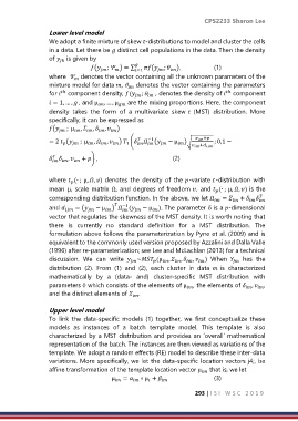
( ;  ) = ∑ ( ; ), (1)

=1
where  denotes the vector containing all the unknown parameters of the

mixture model for data ,  denotes the vector containing the parameters

for component density, ( ;  , denotes the density of component
ℎ
ℎ

= 1, … , , and µ , … , µ are the mixing proportions. Here, the component

density takes the form of a multivariate skew (MST) distribution. More
specifically, it can be expressed as
( ; µ , , , )

= 2 ( ; µ , , ) ( −1 ( − µ )√ + ; 0,1 −

1

+

, + ) , (2)

where (∙ ; µ, , ) denotes the density of the -variate -distribution with

mean µ, scale matrix Ω, and degrees of freedom , and (∙ ; µ, , ) is the

corresponding distribution function. In the above, we let = +

and = ( − µ ) −1 ( − µ ). The parameter δ is a -dimensional

vector that regulates the skewness of the MST density. It is worth noting that
there is currently no standard definition for a MST distribution. The
formulation above follows the parameterization by Pyne et al. (2009) and is
equivalent to the commonly used version proposed by Azzalini and Dalla Valle
(1996) after re-parameterization; see Lee and McLachlan (2013) for a technical
discussion. We can write ~ (µ , , , ) When has the

distribution (2). From (1) and (2), each cluster in data is characterized
mathematically by a (data- and) cluster-specific MST distribution with
parameters  which consists of the elements of µ , the elements of , ,

and the distinct elements of .

Upper level model
To link the data-specific models (1) together, we first conceptualize these
models as instances of a batch template model. This template is also
characterized by a MST distribution and provides an ‘overall’ mathematical
representation of the batch. The instances are then viewed as variations of the
template. We adopt a random effects (RE) model to describe these inter-data
variations. More specifically, we let the data-specific location vectors j4;, be
affine transformation of the template location vector µ that is, we let

µ = ∘ µ + (3)

293 | I S I W S C 2 0 1 9