Page 20 - Contributed Paper Session (CPS) - Volume 5

CPS649 A-Hadi N. Ahmed et al.
1 + +

(; ) = ( ≥ ) = (1 − ) , = 0,1,2, … ∈ (0,1).
1 +
Its hrf reduces to
2
() (2 + )
(; ) = = , = 0,1,2, … ∈ (0,1).
( ≥ ) 1 + +
It is easy to see that lim (; ) = . Hence, the parameter can be
→∞
interpreted as a strict upper bound on the failure rate function, an important
characteristic for lifetime models, corresponding to Equation (1).
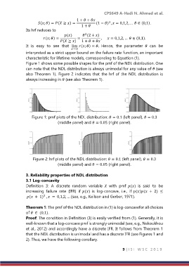
Figure 1 shows some possible shapes for the pmf of the NDL distribution. One
can note that the NDL distribution is always unimodal for any value of (see
also Theorem 1). Figure 2 indicates that the hrf of the NDL distribution is
always increasing in (see also Theorem 1).

Figure 1: pmf plots of the NDL distribution: = 0.1 (left panel), = 0.3
(middle panel) and = 0.05 (right panel).

Figure 2: hrf plots of the NDL distribution: = 0.1 (left panel), = 0.3
(middle panel) and = 0.05 (right panel).

3. Reliability properties of NDL distribution
3.1 Log-concavity
Definition 3: A discrete random variable with pmf () is said to be
increasing failure rate (IFR) if () is log-concave, i.e., if ()( + 2) ≤
( + 1) , = 0,1,2, … (see, e.g., Keilson and Gerber, 1971).
2

Theorem 1: The pmf of the NDL distribution in (1) is log-concavefor all choices
of ∈ (0,1).
Proof. The condition in Definition (3) is easily verified from (1). Generally, it is
well-known that a log-concave pmf is strongly unimodal (see, e.g., Nekoukhou
et al., 2012) and accordingly have a discrete IFR. It follows from Theorem 1
that the NDL distribution is unimodal and has a discrete IFR (see Figures 1 and
2). Thus, we have the following corollary.

9 | I S I W S C 2 0 1 9