Page 361 - Contributed Paper Session (CPS) - Volume 7

CPS2130 Abdul-Aziz A. Rahaman et al.

The M step of EM algorithm is easy to implement in broad classes of problems,
such as in exponential families, since it uses the identical computational
method as ML estimation from L / Y.

3. Result
For the purposes of simplifying and organizing the presentation of results,
the residual parameters presented and discussed here are within the context
of the four categories of estimators being compared.

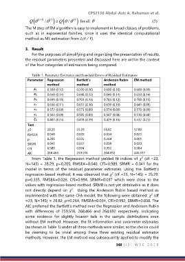
Table 1. Parameter Estimates and Standard Errors of Residual Estimators
Parameter Regression Bartlett’s Anderson Rubin EM method
method method method
0.598 (0.12) 0.599 (0.10) 0.600 (0.10) 0.600 (0.09)
0.648 (0.14) 0.648 (0.13) 0.649 (0.14) 0.650 (0.14)
0.699 (0.15) 0.701 (0.13) 0.703 (0.12) 0.700 (0.15)
0.636 (0.11) 0.637 (0.10) 0.639 (0.10) 0.641 (0.09)
0.572 (0.09) 0.573 (0.09) 0.574 (0.09) 0.578 (0.09)
0.504 (0.09) 0.505 (0.09) 0.507 (0.08) 0.510 (0.08)
0.407 (0.24) 0.418 (0.19) 0.429 (0.16) 0.432 (0.23)
Test
2 28.29 25.29 26.82 57.80
RMSEA 0.040 0.026 0.034 0.023
p 0.205 0.335 0.264 0.001
SRMR 0.041 0.037 0.038 0.020
CFI 0.989 0.994 0.992 0.984
AIC 268.466 259.516 264.692 246.317
From Table 1, the Regression method yielded fit indices of (df =23,
2
N=145) = 28.29, p=0.205, RMSEA=0.040, CFI=0.989, SRMR = 0.041 for the
model in terms of the residual parameter estimates. Using the Bartlett’s
regression-based method, it was observed that (df =23, N=145) = 25.29,
2
p=0.335, RMSEA=0.026, CFI=0.994, SRMR=0.037 which were close to the
values with regression-based method. SRMR is not yet obtainable as it does
not directly depend on . Using the Anderson Rubin based method as
2
implemented with the same CFA model, the following were obtained: (df
2
=23, N=145) = 26.82, p=0.264, RMSEA=0.034, CFI=0.992, SRMR=0.038. The
AIC preferred the Bartlett’s method over the Regression and Anderson Rubin
with differences of 259.516, 268.466 and 264.692 respectively, indicating
some evidence for slightly heavier tails in the sample distributions even
without EM method. However, the fit information and parameter estimates
(as shown in Table 1) under all three methods were similar, so the choice could
be deeming to be trivial among these three existing residual estimator
methods. However, the EM method was subsequently applied to modify the
348 | I S I W S C 2 0 1 9