Page 360 - Contributed Paper Session (CPS) - Volume 7

CPS2130 Abdul-Aziz A. Rahaman et al.

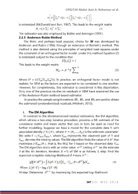
is minimized (McDonald and Burr, 1967). This leads to the weight matrix

The estimator was also employed by Bollen and Arminger (1991).
2.2.3 Anderson-Rubin Method
The third, and perhaps least popular, choice for W was developed by
Anderson and Rubin (1956) through an extension of Bartlett's method. This
method is also derived using the principles of weighted least squares under
the constraint of an orthogonal factor model. Under this method Equation (2)
is minimized subject to the condition that
′
[ ] =

This leads to the weight matrix
−1
−1 ′
= Λ ∑ (3)

2
′ −1
Where = (Λ Σ Σ Σ −1 Λ). In practice, an orthogonal factor model is not

realistic for SEM as the factors are expected to be correlated to one another.
However, for completeness, this estimator is considered in this dissertation.
Only one of the previous studies on residuals in SEM have examined the use
of the Anderson-Rubin method-based estimator.
In practice the sample weight matrices Wr , Wb , and War are used to obtain
the estimated (unstandardized) residuals (Hildreth, 2013).

i. The EM Algorithm
In contrast to the aforementioned residual estimators, the EM algorithm,
which utilizes a two-step iterative procedure, provides a ML estimate of the
covariance matrix and mean vector that can, in turn, be used as input for
further modelling. Suppose we have a model for the complete data Y, with
associated density  /  , where  = ( , … , ) is the unknown parameter.
1

We write   ,  , where represents the observed part of Y and
∗
denotes the missing values. The EM algorithm finds the value of , that
maximizes  /  , that is, the MLE for  based on the observed data Yobs.
The EM algorithm starts with an initial value  . Letting  be the estimate
0
t
 at the ith iteration, iteration (t +1) of EM is as follows; E step: Find the
expected complete-data log-likelihood if  were  :
t

M step: Determine  (t+1) by maximizing this expected log-likelihood:

347 | I S I W S C 2 0 1 9