Page 181 - Special Topic Session (STS) - Volume 3

STS539 Chenglong Li
removed. At any point in time, the process operates in either IC or OC state,
which is only partially observable through 3 sampling or inspection. Let =
[; ;] be the state probability vector of the process at the beginning of the
th
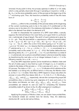
monitoring cycle. Then, the transition probability matrix has the basic
form of
t → t →
= [ ] (3)
t oc→ic t oc→o
where → refers to the probability of the process status at the beginning
of the current monitoring cycle to be in the state of conditioned on the
previous one in the state of . The stationary distribution of a Markov chain is
able to be derived if we obtain the elements of .
In order to characterize the operation of a SPRT chart within a sample,
suppose, the interval between the lower limit and upper limit ℎ is portioned
into subintervals of equal length. The width of each subinterval is given by
∆= (ℎ − )⁄ . Thus, the test statistic experiences different transient states,
i.e., 1 = [, + ∆] , 2 = [ + ∆, + 2∆] , ,, = [ + ( − 1)∆, + ∆] , ,,
= [ + ( − 1)∆, ℎ] , within the control limits before going to an “IC state” (
< ) or an “OC state” ( > ℎ). Assume that the probability density within the
th
subinterval [ + ( − 1)∆, + ∆] for = 1,2, … , is concentrated as a
probability mass at the center, = + ( − 0.5)∆. We further define the two
absorbing states, 0 = [−∞, ] and +1 = [ℎ, +∞], such that there is a total of
+ 2 subintervals. Let us adopt a simplified notation scheme to label the states
by transforming the real value to an integer between 0 and + 1 in the
following manner, for ∈ → = .
Thus, the SPRT inspection system can be modelled as a Markov chain and
the set of states space is described by a pair of integers (, ). A variable, ,
relates to the status of the process: = 0 for a process is IC, and = 1 for an
OC process. The index ∈ {0,1, … ,, … , + 1} indicates which subinterval the
test statistic is falling into, as defined before. In this way, the Markov chain
(, ) has 2 × ( + 2) states. Note that, a SPRT inspection stops only when the

process is in one of the four states: (0,0), (0, + 1), (1,0), (1, + 1). We let (0,0)

, , (1,0) and (1,s+1) , respectively, denote the corresponding expected
(0,s+1)
probabilities when a monitoring cycle originates at IC state and ends at the

four states, and likewise, we have (0,0) , (0,s+1) , (1,0) and . These
(1,s+1)
probabilities are relevant to and are used for computing the transition
probability matrix as shown in Eq. (3), after arrangement resulting in
+ +
= [ (0,0) (0,s+1) (1,s+1) (1,0) ] (4)

+ (0,s+1) + (1,s+1) (1,0)
(0,0)
Applying the property of Markov chain, we can obtain these probabilities.
The technical details are omitted here for brevity. Then, the stationary
distribution ∗ can be derived as follows,
170 |I S I W S C 2 0 1 9