Page 149 - Contributed Paper Session (CPS) - Volume 6

CPS1851 Hee Young Chung et al.
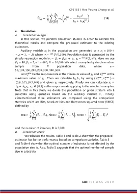
ℎ
1 2
= ∑ ∑ ( () − 1 () ) (14)
̅ ̂
ℎ

0
ℎ=1 =1 +
1

4. Simulation
a. Simulation design
In this section, we perform simulation studies in order to confirm the
theoretical results and compare the proposed estimator to the existing
estimators.
Auxiliary variable in the population are generated with = 100 +

, = 1, ⋯ , where ~ (0,100). Population data is generated by the

2
simple regression model = + + , ~ (0, ). Here we use
0

1
= 10, = 5, = 400, = 10,000. We select n samples by simple random
2
0
1
sample from population data, where n =
50, 100, 150, 200, 250, 300, 400, 500.
Let be the response rate at the minimum value of and at the

maximum value of . Then we calculate , by using ( , ) =

1
0
(0.9, 0.7), (0.7, 0.9) and given respectively. Finally we can calculate =

+ , ∈ [0,1] as the response rate applying to the selected n samples.
1

0
Note that in this study we divide the population or given stratum into L
substrata using quantiles based on the auxiliary variable . Finally,

aforementioned three estimators are compared using the comparison
statistics which are Bias, Absolute bias and Root mean squared error (RMSE)
defined by

1 1 1
̅ ̂
̅ ̂
̅ ̂
̅
̅
̅
Bias ∶ ∑( − ) , Abias ∶ ∑| − | , RMSE ∶ √ ∑( − )
2

=1 =1 =1
and the number of iteration, R is 3,000.
b. Simulation result
We tabulate the results. Table 1 and Table 2 show that the proposed
estimator has better performance based on comparison statistics. Table 3
and Table 4 show that the optimal number of substrata is not affected by the
population size, . Also, Table 5 suggests that the optimal number of sample
size in substrata.

138 | I S I W S C 2 0 1 9