Page 339 - Invited Paper Session (IPS) - Volume 2

IPS273 Tomoki Tokuda et al.

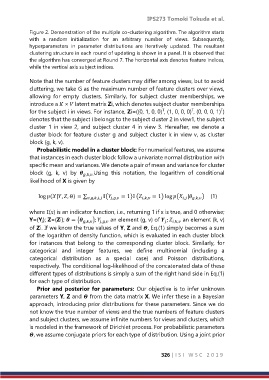
Figure 2. Demonstration of the multiple co-clustering algorithm. The algorithm starts
with a random initialization for an arbitrary number of views. Subsequently,
hyperparameters in parameter distributions are iteratively updated. The resultant
clustering structure in each round of updating is shown in a panel. It is observed that
the algorithm has converged at Round 7. The horizontal axis denotes feature indices,
while the vertical axis subject indices.

Note that the number of feature clusters may differ among views, but to avoid
cluttering, we take G as the maximum number of feature clusters over views,
allowing for empty clusters. Similarly, for subject cluster memberships, we
introduce a × latent matrix Zi, which denotes subject cluster memberships
T
T
T
for the subject i in views. For instance, Zi=((0, 1, 0, 0) , (1, 0, 0, 0) , (0, 0, 0, 1) )
denotes that the subject i belongs to the subject cluster 2 in view1, the subject
cluster 1 in view 2, and subject cluster 4 in view 3. Hereafter, we denote a
cluster block for feature cluster g and subject cluster k in view v, as cluster
block (g, k, v).
Probabilistic model in a cluster block: For numerical features, we assume
that instances in each cluster block follow a univariate normal distribution with
specific mean and variances. We denote a pair of mean and variance for cluster
block (g, k, v) by ,,. Using this notation, the logarithm of conditional
likelihood of X is given by

log (|, , Θ) = ∑ ,,,, ( ,, = 1) ( ,, = 1) log ( | ,, ) (1)
,

where () is an indicator function, i.e., returning 1 if x is true, and 0 otherwise;
Y={Yj}; Z={Zi}; = { ,, }; ,, an element (g, v) of ; ,, an element (k, v)

of Zi. If we know the true values of Y, Z and , Eq.(1) simply becomes a sum
of the logarithm of density function, which is evaluated in each cluster block
for instances that belong to the corresponding cluster block. Similarly, for
categorical and integer features, we define multinomial (including a
categorical distribution as a special case) and Poisson distributions,
respectively. The conditional log-likelihood of the concatenated data of these
different types of distributions is simply a sum of the right hand side in Eq.(1)
for each type of distribution.
Prior and posterior for parameters: Our objective is to infer unknown
parameters Y, Z and from the data matrix X. We infer these in a Bayesian
approach, introducing prior distributions for these parameters. Since we do
not know the true number of views and the true numbers of feature clusters
and subject clusters, we assume infinite numbers for views and clusters, which
is modeled in the framework of Dirichlet process. For probabilistic parameters
, we assume conjugate priors for each type of distribution. Using a joint prior

326 | I S I W S C 2 0 1 9