Page 197 - Special Topic Session (STS) - Volume 1

STS425 Arifah B. et al.
financial time series and it is applied for FTSE Bursa Malaysia KLCI over a period
of 20 years. In this study, we will develop the LSMV model to forecast the CPO
price by using fOU process that have the ability to capture the characteristic
observed in the time series of the CPO. This model is useful to estimate the
degree of its persistency of CPO time series and to simulate the relationship
between the returns and the series volatility. The data will be collected for 12
years daily CPO prices. The drift and diffusion coefficient of the volatility
process are estimated by using the least square estimator (LSE) and quadratic
generalized variations (QGV) methods respectively. The long memory
parameter is estimated by the detrended fluctuation analysis (DFA) method.
This study aims to investigate the CPO prices behavior via the LSMV models.
The model introduce a probabilistic approach in allowing different volatility
states in CPO time series to overcome the excessive persistence problem in
the composite linear and nonlinear models.

2. Methodology
The method of parameters estimation of long memory stochastic volatility
(LMSV) is discussed in this section. At First, the specification of LMSV model
is produced. Then, both the testing methods for the existence of long memory
and the estimation methods of parameters on the drift and diffusion
coefficient of the volatility process are discussed. Finally we assessed the
model performance and the methods of parameters estimation.

2.1 LMSV Model specification
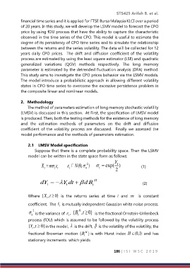
Suppose that there is a complete probability space. Then the LSMV
model can be written in the state space form as follows:
Y
X m   N (0, 2 )   exp( ) (1)
1
t t t t n t
2

dY    Y dt  1  d B t H (2)
1

Where { ,X t  0} is the returns series at time t and m is constant
t
coefficient. The  is mutually independent Gaussian white noise process.
t
 n 2 is the variance of , {B t H ,t  0} is the fractional Ornstein-Unlenbeck
t
process (fOU) which is assumed to be followed by the volatility process
{ ,Y t  0}in the model,  is the drift,  is the volatility of the volatility, the
t
fractional Brownian motion {B t H } is with Hurst index H  (0,1) and has
stationary increments which yields

186 | I S I W S C 2 0 1 9