Page 200 - Special Topic Session (STS) - Volume 1

STS425 Arifah B. et al.
parametric frame of long memory stationary process while in many cases
of trended long range dependent process, the estimator is not converge.
Løvsletten (2017) explored the detrended fluctuation analysis consistency

where () for the stationary and non-stationary stochastic process
with 0 < H < 1 and 1 H  2 respectively.

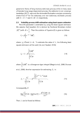
2.3 Volatility process drift estimation using least square estimator
The drift parameter is estimated by using the least square estimator.
We assume that Equation (5) is derived by fractional Brownian motion
1
{B H }with H  . Then the solution of Equation(5) is given as follows
t
2
t
Y    e   (t s ) dB s H , (13)
t
0

0
where y  and   . To estimate the value of  , the following least
0
0
square estimator will be used (Hu and Nualart, 2010):

T
t 
Y dB t H
  T   0 T , (14)
t 
2
Y dt
0

T
t 
H
where Y dB is a divergence-type integral (Biagini et al., 2008, Duncan
t
0
et al., 2000). Another expression for estimating  is :
T

T t
   2H  2  e  d dt
Y 2
 T T T    2 0 0 T , (15)
t 
t 
2
2
2 Y dt Y dt
0 0

Consequently, if

1 T   2 (2H  1)
lim Y dt  t  2 limVar ( )Y  (16)
t t 0 t t 2 2H

Then  can be found as follows:

189 | I S I W S C 2 0 1 9