Page 202 - Special Topic Session (STS) - Volume 1

STS425 Arifah B. et al.

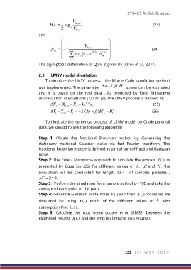
1 V 2
H N  log N ,a , (23)
2 2 V N ,a
and
 
 V 
  N   2 N ,a .  (24)
   a a k  k 2H N  2H N  
N
 , k 
The asymptotic distribution of QGV is given by (Chen et al., 2017).

2.5 LMSV model simulation
To simulate the LMSV process, , the Monte Carlo simulation method
was implemented. The parameter   ( , , H  ) is now can be estimated
and it is based on the real data . As produced by Euler Maruyama
discretization in Equations (1) and (2), The LMSV process is defined as:
i Y
X i  X i 1  X  ke  (25)
/2
i
i
 Y  Y  Y    Y t    (B  B H ) (26)
H
i
i t
1
i
i
i
i t 
1
To illustrate the numerical process of LSMV model on Crude palm oil
data, we should follow the following algorithm

Step 1: Obtain the fractional Brownian motion by Generating the
stationary fractional Gaussian noise via fast Fourier transform. The
fractional Brownian motion is defined as partial sum of fractional Gaussian
noise.
Step 2: Use Euler- Maruyama approach to simulate the process (.)Y as
presented by Equation (26) for different values of ,  and H the
.
simulation will be conducted for length t  1 of samples particles ,
nT  2^9.
Step 3: Perform the simulation for a sample path of p=100 and take the
average of each point of the path.
Step 4: Generate Gaussian white noise (.)Y and then X (.) processes are
simulated by using Y (.) result of for different values of k with
assumption that k  1.
Step 5: Calculate the root mean square error (RMSE) between the
estimated returns X (.) and the empirical returns (log returns).

191 | I S I W S C 2 0 1 9