Page 383 - Special Topic Session (STS) - Volume 2

STS506 L. Leticia R. et al.
“memory” of its hidden state about previously seen sequences (Figure 1a).
These features are combined with the structural properties of the pertaining

graph ( , … , ) and feed into a dense layer that generates the model’s
1

prediction (Figure 1a). is modified to consider the contact network structure
or network topology, as constant variables (Figure 1b).

3. Result
3.1 Exact simulations
To assess the ABC and the proposed modifications, we recreate two set of
synthetic data on epidemics evolving in two different random networks (each
with 500 vertices) with degree distribution: (A) Poisson (2.42) (B)
Polylogarithmic (0.1, 2). For each network we simulate the outbreak
surveillance information using parameter values = 0.03 and = 0.01, and
initial states ((0), (0), (0)) = ( − 2, 2, 0). The generated data is then set “real
data”. As Dutta, et al. (2018), we assume the knowledge on the number of
initial cases in and but we do not specify the individuals in these states. In
contrast with Dutta, et al. (2018), we perform the statistical inference only from
the surveillance-like reports.
The ABC-MCMC described in Section 2.2 is implemented with discrepancy
measure
( − ) 2
(, ) = ∑ √ ( > 0) + ( = 0) ,

where > 0 is a small constant introduced to define (, ) beyond the
observed outbreak span.
We use a Gaussian kernel function and the proposal distribution
corresponds to a mixture of Gaussian densities. This allows to include two
distributions with different standard deviations (in our case, 0.005 and 0.1) to
improve the parametric space exploration. For these experiments, we consider
that and have independent prior exponential distribution with parameters
3, that is equivalent to be approximately 95% confident that each of the real
values are between 0 and 1. After removing the burn-in and thinning the
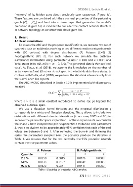
series, the parameters sampled from the posterior produce the statistics in
Table 1. We observe that for the two networks, the 95% posterior intervals
contain the true parameter values.

A: Poisson B: Polylogarithmic
Quantile

2.5 % 0.0250 0.0015 0.0176 0.0008

50 % 0.0333 0.0127 0.0249 0.0085
97.5 % 0.0622 0.0341 0.0411 0.0269

Table 1 Statistics of posterior ABC samples.
372 | I S I W S C 2 0 1 9