Page 182 - Special Topic Session (STS) - Volume 3

STS539 Chenglong Li
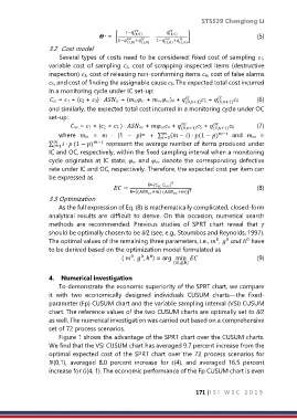
1−
(1,0)
(1,0)
= [ ] (5)
∗
1− + 1− +
(1,0) (1,0) (1,0) (1,0)
3.2 Cost model
Several types of costs need to be considered: fixed cost of sampling 1,
variable cost of sampling c2, cost of scrapping inspected items (destructive
inspection) 3, cost of releasing non-conforming items 4, cost of false alarms
5, and cost of finding the assignable cause 6. The expected total cost incurred
in a monitoring cycle under IC set-up:

= 1 + (2 + 3) ∙ + ( + )4 + (0,s+1) 5 + (1,s+1) 6 (6)

and similarly, the expected total cost incurred in a monitoring cycle under OC
set-up:

= 1 + (2 + 3 ) ∙ + 4 + (0,s+1) 5 + (1,s+1) 6 (7)
where = ∙ (1 − ) + ∑ ( − ) ∙ (1 − ) − and =

=1
∑ ∙ (1 − ) − represent the average number of items produced under
=1
IC and OC, respectively, within the fixed sampling interval when a monitoring
cycle originates at IC state; and denote the corresponding defective
rate under IC and OC, respectively. Therefore, the expected cost per item can
be expressed as
T
Θ∗[ ]
= (8)
Θ∗[( +) ( +)] T
3.3 Optimization
As the full expression of Eq. (8) is mathematically complicated, closed-form
analytical results are difficult to derive. On this occasion, numerical search
methods are recommended. Previous studies of SPRT chart reveal that
should be optimally chosen to be ⁄2 (see, e.g., Stoumbos and Reynolds, 1997).
The optimal values of the remaining three parameters, i.e., , ℎ have
0
0
0
to be derived based on the optimization model formulated as
( , , ℎ ) = arg min (9)
0
0
0
(m,g,h)

4. Numerical investigation
To demonstrate the economic superiority of the SPRT chart, we compare
it with two economically designed individuals CUSUM charts—the fixed-
parameter (Fp) CUSUM chart and the variable sampling interval (VSI) CUSUM
chart. The reference values of the two CUSUM charts are optimally set to ⁄2
as well. The numerical investigation was carried out based on a comprehensive
set of 72 process scenarios.
Figure 1 shows the advantage of the SPRT chart over the CUSUM charts.
We find that the VSI CUSUM chart has averaged 9.7 percent increase from the
optimal expected cost of the SPRT chart over the 72 process scenarios for
(0,1), averaged 8.0 percent increase for (4), and averaged 16.5 percent
increase for (4, 1). The economic performance of the Fp CUSUM chart is even

171 |I S I W S C 2 0 1 9