Page 108 - Special Topic Session (STS) - Volume 4

STS566 K. Prokopenko et al.
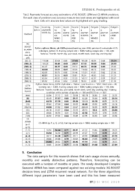
Tab.2. Payments forecast accuracy estimations of XG BOOST, LSTM and CS ARMA predictors.
For each class of predictors and accuracy measure two best values are highlighted with bold
font. Cells with absolute best values are highlighted with gray shading.

Descr Incoming Incomi Incomi Incomi Outgoin Outgoin Outgoin Outgoin
iption payments ng ng ng g g g g
MAPE (%) payme payme payme paymen paymen paymen payment
Method
nts nts R2 nts ts MAPE ts ts R2 s RSD
NRMS RSD (%) NRMSD (%)
D (%) (%) (%)
XG
BOOST
(n_estim Python xgBoost library, gb.XGBRegressor(learning_rate=0.08, gamma=0, subsample=0.75,
colsample_bytree=1), training sample size = 1004, testing sample size = 180, date
ators,
max_de features: “month, month day, year week, month week, week day, working day”
pth)
(50, 2) 170.58 39.68 0.60 27.66 105.68 40.94 0.60 23.24
(100, 2) 103.20 38.43 0.63 28.37 57.13 39.35 0.64 25.53
(100, 3) 64.47 38.17 0.63 29.13 66.73 39.08 0.65 25.63
(100, 4) 60.98 38.89 0.61 30.25 114.63 40.13 0.63 26.32
(100, 5) 62.69 39.75 0.60 31.46 113.51 41.01 0.62 27.16
(250, 3) 62.51 39.35 0.61 30.81 78.54 40.95 0.62 27.21
(500, 3) 62.64 40.32 0.59 32.23 143.17 42.37 0.59 28.57
(500, 5) 85.52 42.66 0.54 35.65 70.24 43.99 0.57 31.15
Python Keras library, LSTM. Optimizer = “Adam”, Loss function = “MSE”, Batch size = 20,
LSTM
learning rate = 0.005, training sample size = 1004, testing sample size = 180, date
(hidden features: “month, month day, year week, month week, week day, working day”, training
layers)
condition: while number of epochs <= 100 and EVS Error <= 0.81
(4x4) 66.94 37.72 0.65 29.58 185.78 36.86 0.69 26.35
(8) 45.49 37.57 0.65 29.11 62.20 35.84 0.72 26.14
(8x8) 44.78 37.70 0.65 29.26 105.04 35.70 0.71 26.19
(16) 45.64 37.94 0.64 29.35 46.69 35.93 0.71 26.18
(16x16) 44.96 37.82 0.64 29.67 226.64 36.05 0.71 26.14
(32) 46.10 37.87 0.64 29.33 49.53 35.8 0.71 26.08
(64) 49.66 38.39 0.63 29.86 42.56 36.65 0.70 26.92
(128) 46.53 37.93 0.64 29.89 62.95 36.96 0.69 26.58
CS
ARMA CS ARMA (p, P, q, Q, L=52), training sample size = 1004, testing sample size = 180
(p=P,
q=Q)
(1, 1) 36.94 34.44 0.71 28.91 47.22 31.86 0.78 28.23
(2,1) 36.92 34.50 0.71 28.99 47.27 31.91 0.78 28.29
(2, 2) 38.17 34.49 0.71 29.11 47.93 31.44 0.78 27.73
(3, 3) 38.68 34.88 0.70 29.64 46.64 31.95 0.78 28.27
(3, 1) 36.86 34.52 0.71 29.05 47.14 31.92 0.78 28.32
(1, 3) 38.65 34.64 0.71 29.30 46.13 31.68 0.78 27.94

5. Conclusion
The data sample for this research shows that cash usage shows annually,
monthly and weekly distinctive patterns. Therefore, forecasting can be
executed with a horizon of months or years. The newly developed Complex
Seasonal ARMA has been compared against two existing models: XG BOOST
decision trees and LSTM recurrent neural network. For the three algorithms
different input parameters have been used and this has been measured

97 | I S I W S C 2 0 1 9