Page 106 - Special Topic Session (STS) - Volume 4

STS566 K. Prokopenko et al.

= + ∑( − − ) + ∑( −− − ) + , > + (, ) (3)

=1 =1

where = 1, … ,7 is a weekday number, is a constant, and are the

order and coefficients of w-weekday’s coefficient autoregressive model,
, and are the order, coefficients and lag of seasonal part of w-weekday’s

coefficient autoregressive model, is white noise.

According to the theory of autoregressive processes [2], parameters
, … , , , … , , , … , , , … , , can be estimated by solving the

1
1

1

1
system of linear equations composed from weekly totals and daily cash
payment turnovers. Forecasting expression for daily payment value + is the
following:
(+) 7+1
+ = (+) 7+1 ∗ (+) 7+1 (4)

and (+) 7+1 were calculated according to (2), (3)
where (+) 7+1 (+) 7+1

4. Experimental results validation
Validation of the CSARMA model was provided on payments data sets
obtained from 100 branches. Each branches data sample has 3 years (1184
days) of both incoming and outgoing payments history. Train sample size =
1004 days, test sample size = 180 days. Error measures are explained in
(Tab.1.).
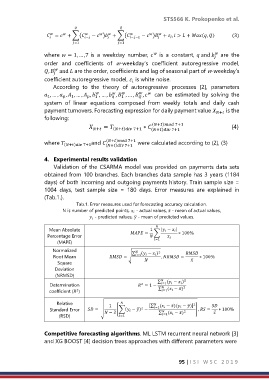
Tab.1. Error measures used for forecasting accuracy calculation.
N is number of predicted points, - actual values, ̅ - mean of actual values,
- predicted values, ̅ - mean of predicted values.

Mean Absolute 1 | − |
Percentage Error = ∑ ∗ 100%
(MAPE) =1
Normalized 2
Root Mean = √ ∑ =1 ( − ) , = ∗ 100%
Square ̅
Deviation
(NRMSD)
∑ ( − ) 2
Determination = 1 − =1 2
2

coefficient ( ) ∑ =1 ( − ̅)
2
Relative [∑ ( − ̅)( − ̅)] 2
Standard Error = √ 1 [∑( − ̅) − =1 2 ] , = ∗ 100%
2
(RSD) − 2 =1 ∑ =1 ( − ̅) ̅

Competitive forecasting algorithms. ML LSTM recurrent neural network [3]
and XG BOOST [4] decision trees approaches with different parameters were
95 | I S I W S C 2 0 1 9