Page 138 - Contributed Paper Session (CPS) - Volume 1

CPS1201 M. Iftakhar Alam et al.
2
̃
() = , Θ,
( − ) 2
2
1 2
3
where
Θ = {: < ≤ < , 0 < ≤ , 0 < ≤ }
̃
3
3
2
1
2
2
4
1

The associated FIM (, ) for the model parameters can be obtained easily.

Simulation settings
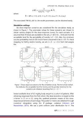
Six dose-response scenarios are considered for the simulation study, as
shown in Figure 1. The parameter values for these scenarios are chosen to
obtain various shapes for the dose-response curves. For each scenario, it is
assumed that 20 doses are available in the set = {0.5,1.0,...,10.0} and that the
acceptable level for the probability of toxicity is Υ = 0.2. Also, the minimum
success probability that an OD should have is assumed to be δ = 0.5. To check
stopping for futility and/or toxicity, we set = − = 0.3. Each trial assigns
the

Figure 1: Dose-response scenarios for the simulation study. The horizontal dashed
line indicates the acceptable level for toxicity and the penalty functions for the
scenarios are obtained assuming that CS = CT = 1.

lowest available dose of 0.5 mg/kg body weight to a cohort of patients. After
obtaining responses from the first cohort, the dose escalation is based on the
criterion in (1) or in (2), using the updated posterior means of the dose-
response parameters at each stage. The posterior means are obtained through
numerical integration using the R package cubature (Johnson and
Narasimhan, 2013). We use a joint uniform prior distribution for . The

127 | I S I W S C 2 0 1 9