Page 179 - Contributed Paper Session (CPS) - Volume 2

CPS1496 Tim Christopher D.L et al.
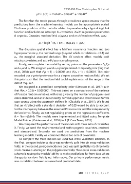
p2i ∶ () = 2.616 − 3.596 + 1.594
3
2
The fact that the model passes through prevalence space ensures that the
predictions from the machine learning models can be appropriately scaled.
The linear predictor of the model is related to prevalence by a typical logit link
function and includes an intercept, β0, covariates, X with regression parameters
β, a spatial, Gaussian, random field, u(s,ρ,σu), and an iid random effect, vj(σv).

−1
pb = logit (β0 + βX + u(s,ρ,σu) + vj(σv))
The Gaussian spatial effect has a Mat´ern covariance function and two
hyperparameters: ρ, the nominal range (beyond which correlation is < 0.1) and
σu, the marginal standard deviation. The iid random effect models both
missing covariates and extra-Poisson sampling error.
Finally, we complete the model by setting priors on the parameters β0,β,ρ
and σu and σv. We assigned ρ and σu a joint penalised complexity prior (Fuglstad
et al., 2018) such that P(ρ < 1) = 0.00001 and P(σu > 1) = 0.00001. This prior
encoded our a priori preference for a simpler, smoother random field. We set
this prior such that the random field could explain most of the range of the
data if required.
We assigned σv a penalised complexity prior (Simpson et al., 2017) such
that P(σv > 0.05) = 0.0000001. This was based on a comparison of the variance
of Poisson random variables, with rates given by the number of polygon-level
cases observed, and an independently derived upper and lower bound for the
case counts using the approach defined in (Cibulskis et al., 2011). We found
that an iid effect with a standard deviation of 0.05 would be able to account
for the discrepancy between the assumed Poisson error and the independently
derived error. Finally, we set regularising priors on the regression coefficients
βi ∼ Norm(0,0.4). The models were implemented and fitted using Template
Model Builder (Kristensen et al., 2016) in R (R Core Team, 2018).
We compared the performance of the models with three sets of covariates,
X. Firstly, we used the environmental and anthropogenic covariates, centered
and standardised. Secondly, we used the predictions from the machine
learning models. Finally we combined these two sets of covariates.
To compare the three models we used two cross-validation schemes. In
the first, polygon incidence data was randomly split into six cross-validation
folds. In the second, polygon incidence data was split spatially into three folds
(via k-means clustering on the polygon centroids). This spatial cross-validation
scheme is testing the models' ability to make predictions far from data where
the spatial random field is not informative. Our primary performance metric
was correlation between observed and predicted data.

168 | I S I W S C 2 0 1 9