Page 305 - Contributed Paper Session (CPS) - Volume 2

CPS1871 Natividad J.M. et al.
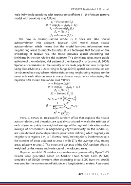
male individuals associated with regression coefficient , the Poisson-gamma
1
model with covariate is as follows:
~ ( )

= exp( + + )

0
1 1

~ ( , )
1
1

~ ( )
0
~ (1,1).
1
The flaw in Poisson-Gamma model is it does not take spatial
autocorrelation into account. Bayesian CAR model allows spatial
autocorrelation which means that the model borrows information from
neighboring areas to smooth the rates. It is a technique that focuses on the
smoothing of relative risk. The model provides spatial smoothing and
shrinkage in the raw relative risk estimate. This shrinkage gives more stable
estimate of the underlying risk pattern of the disease (Richardson et. al., 2004).
Spatial autocorrelation in the sexually active male population was computed
using Global Moran’s I. According to Tango (2010), spatial autocorrelation can
be observed in a way where relative risks among neighboring regions are the
same with each other as seen in many disease maps hence introducing the
Bayesian CAR model. The model is as follows:
~ ( )

= exp( + + )

1 1
0

~ ( )
0
~ (1,1)
1
1
2
| ≠ ~ (̅̅̅, )

1
̅ = ∑

∑ =1
=1
2
2
= .

∑
=1
Here, serves as area-specific random effect that explains the spatial

autocorrelation, and the priors are spatially structured wherein the estimate of
each city/municipality is a weighted average of the regional data value and an
average of observations in neighboring city/municipality. In this model,

are user-defined spatial dependence parameters defining which regions j are
neighbors to regions i; = 1 if areas i and j are neighbors, 0 otherwise; is

the number of areas adjacent to area i while ̅̅̅ is the average of among

areas adjacent to area i. The mean and variance of the CAR random effect is
weighted by the means and variances of the adjacent areas.
Bayesian models HIV incidence estimates were generated by OpenBUGS.
Results were generated based on Markov Chain Monte Carlo (MCMC)
simulation of 30,000 iterations after discarding initial 3,000 burn-ins. ArcGIS
was used for the conversion of latitude and longitude into meters. R was used
294 | I S I W S C 2 0 1 9