Page 155 - Contributed Paper Session (CPS) - Volume 3

CPS1979 Francisco N. de los R.
~(0,1)
The random effects = ( , . . . , ) shall account for the spatial dependence
1

in the data, and are represented by a CAR prior distribution. Moran’s Index
was used to confirm if spatial autocorrelation exists. The CAR priors shall
induce the spatial autocorrelation by a binary × proximity matrix
= ( ), which is computed from the contiguity structure of the areal

units. Based on , the CAR priors take the form of a zero-mean multivariate
Gaussian distribution, where spatial autocorrelation is induced via the
precision matrix that depends on W. Leroux et al. (1999) proposed that the
strength of the autocorrelation be estimated from the data. The precision
matrix for this model involves an autocorrelation parameter and the proximity
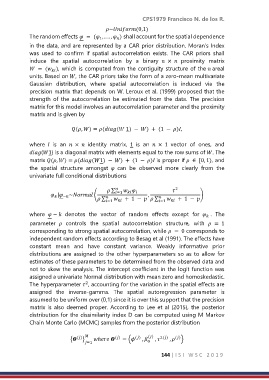
matrix and is given by

(, ) = (( 1) − ) + (1 − ),

where is an × identity matrix, 1 is an × 1 vector of ones, and
(1) is a diagonal matrix with elements equal to the row sums of . The
matrix (, ) = ((1) − ) + (1 − ) is proper if ∈ [0, 1), and
the spatial structure amongst can be observed more clearly from the
univariate full conditional distributions

∑ 2
| ~ ( =1 , )
−

∑ + 1 − ∑ + 1 −

=1
=1

where − denotes the vector of random effects except for . The

parameter controls the spatial autocorrelation structure, with = 1
corresponding to strong spatial autocorrelation, while = 0 corresponds to
independent random effects according to Besag et al (1991). The effects have
constant mean and have constant variance. Weakly informative prior
distributions are assigned to the other hyperparameters so as to allow for
estimates of these parameters to be determined from the observed data and
not to skew the analysis. The intercept coefficient in the logit function was
assigned a univariate Normal distribution with mean zero and homoskedastic.
The hyperparameter , accounting for the variation in the spatial effects are
2
assigned the inverse-gamma. The spatial autoregression parameter is
assumed to be uniform over (0,1) since it is over this support that the precision
matrix is also deemed proper. According to Lee et al (2015), the posterior
distribution for the dissimilarity index D can be computed using M Markov
Chain Monte Carlo (MCMC) samples from the posterior distribution

{ () } ℎ () = ( () , () , 2() , () )
=1 0
144 | I S I W S C 2 0 1 9