Page 42 - Contributed Paper Session (CPS) - Volume 3

CPS1941 Jang S.
The disturbance terms for the three groups are = 33.11, = 54.18
1
2
and = 78.85 respectively. The dispersion is thus higher in the groups with
3
higher salaries then in those with lower salaries. This makes sense, since in the
low salary group a lot of employees just earn the minimal wage. Hence, a lot
of them have the same salary.
Moreover this example illustrates the dependence of the trajectories on
Luxembourg’s GDP. We see that in the three groups, this influence is non
linear, since is always significantly different from 0. The trajectory equations
2
from table 1 can now be used to predict the future evolution of the salaries
for men and women as a function of GDP.

5. Model Selection in Finite Mixture Models
Till now, there has been no really satisfactory solution for a model selection
procedure, in the sense of addressing the challenge to determine the optimal
number of classes in a family of finite mixture models. Nagin (2005)
emphasizes the need of an interplay of formal statistical criteria and subjective
judgment and proposes to use the Bayesian Information Criterion (BIC),
defined by

BIC = log() − 0, 5 log(), (6)

where denotes the number of parameters in the model. The bigger the BIC,
the better the model explains the data. The correction term 0.5 log() is
necessary, because the likelihood is an increasing function of the number of
groups and just taking the likelihood as criterion does hence not make any
sense.
Nielsen et al. (2014) argue that the existing software does not always
compute the BIC accurately and that furthermore BIC on its own does not
always indicate a reasonable-seeming number of groups even when
computed correctly. They propose the methodology of cross-validation error
(CVE) instead, which consists in computing a CVE for each possible choice r of
the number of latent classes, indicating the extent to which the model fails to
perfectly model the data. The final choice of r is then the one that minimizes
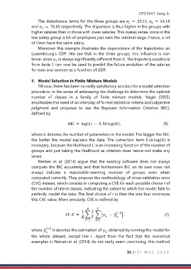
this CVE value. More precisely, CVE is defined by

1 1
= ∑ ∑ | − ̂ [−] |, (7)

−1 =1

[−]
where ̂ it denotes the estimation of obtained by running the model for

the whole dataset, except line . Apart from the fact that the numerical
examples in Nielsen et al. (2014) do not really seem convincing, this method

31 | I S I W S C 2 0 1 9