Page 37 - Contributed Paper Session (CPS) - Volume 3

CPS1941 Jang S.
we discuss model selection and group member probabilities for the new
model. In section four, we highlight typical features of the new model by
means of a data example from economics. In section five, finally, we introduce
the classical criteria for determining the optimal number of trajectory groups
in finite mixture models and propose a new criterion which does not need a
lot of computer power to compute, even in case of large samples and does
not depend on the number of parameters of the model.

2. Nagin's Finite Mixture Model
Starting from a collection of individual trajectories, the aim of Nagin’s finite
mixture model is to divide the population into a number of homogenous sub-
populations and to estimate, at the same time, a typical trajectory for each
sub-population (Nagin 2005). More, precisely, consider a population of size N
and a variable of interest Y. Let = , , … , be T measures of the
2
1

variable Y, taken at times , … , for subject number . To estimate the
1

parameters defining the shape of the trajectories, we need to fix the number
of desired subgroups. Denote the probability of a given subject to belong to
group number by .

The objective is to estimate a set of parameters

Ω = { , , , … ; = 1, … , } which allow to maximize the probability of the

01
0
measured data. The particular form of Ω is distribution specific, but the
parameters always perform the basic function of defining the shapes of the
trajectories. In Nagin’s finite mixture model, the shapes of the trajectories are
described by a polynomial function of age or time. In this paper, we suppose
that the data follow a normal distribution. Assume that for a subject in
group

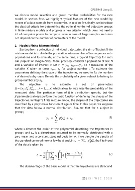
= ∑ + (1)

=1

where denotes the order of the polynomial describing the trajectories in
group and is a disturbance assumed to be normally distributed with a

zero mean and a constant standard deviation . If we denote the density of

the standard centered normal law by and = ∑ =1 , the likelihood

of the data is given by

1 − (2)

= ∏ ∑ ∏ ( ).

=1 =1 =1

The disadvantage of the basic model is that the trajectories are static and
26 | I S I W S C 2 0 1 9