Page 131 - Contributed Paper Session (CPS) - Volume 4

CPS2156 Luis Sanguiao Sande
bias removal. A weighted mean is taken over all possible divisions of the
sample, so that the estimator becomes design unbiased. We get the weights
from what we will call a two stage decomposition.

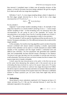
Definition 1: Let 1, 2 a two stage sampling design, where 2 depends on
the first stage sample denoted by 1. (1,2) is said to be a two stage
decomposition of if and only if

() = ∑ ( ) (\ )
1
1
2
1
⍛⊂
for any sample .
Suppose is just simple random sampling of size . An example of two
stage decomposition is a simple random sampling of size − 1 and a simple
random sampling of size 1 on the remaining units. For simplicity, this is the
decomposition we are going to use in the examples. Of course, the
decomposition is not unique, even if we fix and the sample size of both 1
and 2 . The optimal choice of a decomposition is still an open problem.
The first sample 1 will be used for modeling and the second one \1 for
Horvitz-Thompson estimation [3] of the difference between the model and the
target variable.
In the examples, the machine learning algorithm used is random forest [2],
because combined with simple random sampling a simpler, approximate
version of the estimator can be used [5]. In both examples we extract 10000
samples of the population and the target variable is estimated with and
without bias correction. The first population was generated with synthetic
data, and unexpectedly the bias removal causes a decrease in the variance.
The second one uses real data, but the population is not the real one but a
small subsample. This time we have a variance increase, but the increase in the
square mean error is barely noticeable.
In both cases the bias removal seems to be useful: in the first one we are
at the same time decreasing the variance and in the second one we are
eliminating the bias at almost no cost on the square mean error. Of course,
some questions arise. Is there an optimum two stage decomposition? When
should we expect a variance decrease and when an increase? When should we
expect an important increase of the square mean error? We have no definitive
answers to these questions yet, but some ideas that might help will be
discussed.

2. Methodology
What follows is more extensively explained in [5]. Suppose we have a 2
based estimator of . We use the subscript because 2 (and thus the
̂
1
estimator) depends on the sample 1.

120 | I S I W S C 2 0 1 9