Page 132 - Contributed Paper Session (CPS) - Volume 4

CPS2156 Luis Sanguiao Sande
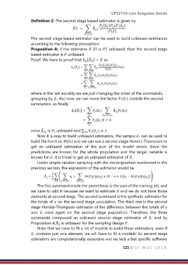
Definition 2: The second stage based estimator is given by
( ) (\ )
̂
2 = ∑ ̂ 1 1 2 1
1
()
⍛⊂
The second stage based estimator can be used to build unbiased estimators
according to the following proposition.
Proposition A: If the estimator 1 is 2 unbiased, then the second stage
based estimator is unbiased.
Proof. We have to proof that ( ) = so
̂

2

where in the last equality we are just changing the order of the summands,
grouping by 1. But now, we can move the factor 1(1) outside the second
summation, so finally

since is 2 unbiased and ∑ ( ) = 1.
̂
1
1
1
1
Now it is easy to build unbiased estimators. The sample 1 can be used to
build the function (1) and we can use a second stage Horvitz-Thompson to
get an unbiased estimation of the sum of the model errors. Since the
predictions are known for the whole population and the target variable is
known for 1 it is trivial to get an unbiased estimator of .
Under simple random sampling with the decomposition mentioned in the
previous section, the expression of the estimator would be

The first summand inside the parenthesis is the sum of the training set, and
we have to add it because we want to estimate and we do not have those
elements at second stage. The second summand is the synthetic estimator for
the totals of on the second stage population. The third one is the second
stage Horvitz-Thompson estimator of the difference between the totals of
and , once again on the second stage population. Therefore, the three
summands compound an unbiased second stage estimator of , and by
Proposition A, is unbiased for the sampling design .
̂
2
Note that we have to fit a lot of models to build these estimators: even if
2 contains just one element, we will have to fit models! So second stage
estimators are computationally expensive and we lack a fast specific software

121 | I S I W S C 2 0 1 9