Page 230 - Contributed Paper Session (CPS) - Volume 4

CPS2203 Thierry D. et al.
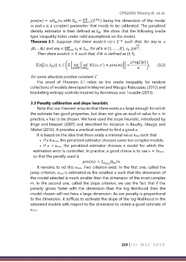
() = /, with = ∑ (2 | | ) being the dimension of the model
=1

and is a constant parameter that needs to be calibrated. The penalized
density estimator is then defined as . We show that the following oracle
̂
type inequality holds under mild assumptions on the model.
Theorem 3.1. Suppose that there exists 0 <∈< 2 − such that, for any =

(B1,...,BK) and any s=∏ ∈ , for all ∈ {1, … . , }, ≥∈ .

=1
Then there exists > 0 such that, if ̂ is defined as (3.1),
log(2)
2
∗
[ (, )] ≤ ( [ inf { inf (, ) + ()}] + ), (3.2)
̂

∈ ̂ ∈
for some absolute positive constant C
The proof of Theorem 3.1 relies on the oracle inequality for random
collections of models developed in Meynet and Maugis-Rabusseau (2012) and
bracketing entropy controls inspired by Bontemps and Toussile (2013).

3.3 Penalty calibration and slope heuristic
Note that our theorem ensures that there exists a κ large enough for which
the estimate has good properties, but does not give an explicit value for κ. In
practice, κ has to be chosen. We have used the slope heuristic, introduced by
Birgé and Massart (2007) and described for instance in Baudry, Maugis and
Michel (2012). It provides a practical method to find a good κ.
It is based on the idea that there exists a minimal value κmin such that
• if κ ≤ κmin, the penalized estimator chooses some too complex models,
• if κ > κmin, the penalized estimator chooses a model for which the
estimation error is controlled. In practice, a good choice is to use κ = 2κmin
so that the penalty used is
/.
() = 2
It remains to nd this κmin. Two criterion exist. In the first one, called the
jump criterion, κmin is estimated as the smallest κ such that the dimension of
the model selected is much smaller than the dimension of the most complex
m. In the second one, called the slope criterion, we use the fact that if the
penalty grows faster with the dimension than the log likelihood then the
model chosen will not have a large dimension. As our penalty is proportional
to the dimension, it suffices to estimate the slope of the log likelihood in the
saturated models with respect to the dimension to obtain a good estimate of
κmin.

219 | I S I W S C 2 0 1 9