Page 101 - Contributed Paper Session (CPS) - Volume 5

CPS1111 Jitendra Kumar et al.
3.1 Estimation under Classical Framework
Present section considers well known regression based method namely,
classical least square estimator (OLS). To make M-AR model more compact,
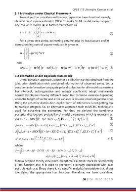
one can write model (4) in further matrix form as
    

Y  l X Z      W    (5)

 
  
For a given time series, estimating parameter(s) by least square and its
corresponding sum of square residuals is given as
   ˆ 

ˆ
1
ˆ
      WW   W  (6)
Y
 
ˆ
 
 
and


ˆ
ˆ
SSR   Y  W   Y  W   Y  W W  W  W  Y   Y  W W  W  W  Y  (7)

1
1

3.2 Estimation under Bayesian Framework
Under Bayesian approach, posterior distribution can be obtained from the
joint prior distribution with combined information of observed series. Let us
consider an informative conjugate prior distribution for all model parameters.
For intercept, autoregressive and merger coefficient, adopt multivariate
normal distribution having different mean but common variance depending
upon the length of vector and error variance is assume inverted gamma prior.
Using the posterior distribution, explicit form of estimators is not getting due
to multiple integrals. So, an alternative approach such as MCMC technique is
used for obtaining the estimators. For that, we derived the conditional
posterior distribution/ probability of model parameters which is represent as
 
'
'
'
  , , 2 , y ~ MVN    Y  X   Z   l   I 2 1    I  2 1  1 '  I 2  1  1  2 (8)
  , l l
l l
2


1
1
  , , 2 , y ~ MVN    Y l   Z   X   I p  1 1  2 p X ' X  I  p 1 1  2 p   , X ' X  I  p 1 1  2 p   (9)

'
'


1
1
'
  , , 2 , y ~ MVN    Y l   X   Z   I R 1   Z  I R 1    , Z ' Z  I R 1    (10)
'
2

'
Z

 2  ,  , , y ~ IG  T  R  p 1  p 2  a  ,1 S   (11)
 2 
where
1
S   Y  l  X  Z  Y  l  X  Z       I 1     
'
'
2 2
'
     I p 1  p 2          I R 1     2  b
1 
'
From a decision theory view point, an optimal estimator must be specified by
a loss function and it is used to represent a penalty associated with each
possible estimate. Since, there is no specific analytical procedure that allows
identifying the appropriate loss function. Therefore, we have considered
90 | I S I W S C 2 0 1 9