Page 15 - Contributed Paper Session (CPS) - Volume 7

CPS2014 Ma. S.B.P. et al.
through a backfitting algorithm) incorporating the VAR(1) model estimation
illustrated in Algorithm 1 and the GAM procedure which involves the
implementation of the backfitting algorithm and the General Local Scoring
Algorithm, and (2) Algorithm 3 (sieve bootstrap on the bivariate residual
matrix).

Algorithm 1: () to estimate the output vector autocorrelation
coefficient
The vector autoregression (VAR) model is one of the most successful,
flexible, and easy to use models for the analysis of multivariate time series. The
VAR model is useful in describing the dynamic behavior of economic and
financial time series (Zivot and Wang, 2006).
′
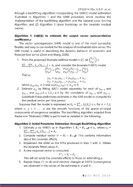
1. From the proposed bivariate additive model in [2], let ( 1 ) =
2 ′
∑ ∑ ( ,− ) + and consider the bivariate (1) model

,
=1
=1

( 1 ) = ( 11 12 ) ( 1−1 ) + ( 1 )

2
21
2−1
22
2
That is,
1 = + + 1
12 2−1
11 1−1
2 = + + 2
22 2−1
21 1−1
where , 21 ≠ 0 and ( , ) = 12 ≠ 0.
1
2
12
2. Estimate by fitting (1) model separately for each of 1−1 and

2−1 and , , = 1,2, ≠ by the correlation of 1−1 with 2−1 .

Substitute these preliminary estimates in the VAR model to compute for
the residual vector per time period.
Suppose that the model is expressed as = ∑ ( ) + , for ℎ = 1,2,
ℎ

=1
where , , = 1, … , are the smooth functions of the sparse principal
components of exogenous variables. The backfitting algorithm adapted from
Hastie and Tibshirani (1986) is performed as detailed in the following.

Algorithm 2: Initial Parameter Estimation through Backfitting Algorithm
1. Estimate by VAR(1) as in Algorithm 1: = − + , where =

∑ ∑ ( ,− ) + .

,
=1
=1
2. Compute residual vector = − − . This contains information
about the covariate effects.
3. Implement the GAM on the SPCs produced in Step 1 with . Obtain
the bivariate fitted values .
4. A new response vector is computed,
∗ = − .

This will set aside the covariate effects to focus on estimating .
5. Repeat Steps (1) to (4) until minimal changes at 0.01% (convergence)
are observed in the values of the estimates in ̂ and .
4 | I S I W S C 2 0 1 9