Page 25 - Contributed Paper Session (CPS) - Volume 7

CPS2020 Honeylet T. S.
2.2. Estimation of the Model
The goal of this study is to estimate a model of variable Y using variable
Z after matching. The model is Poisson loglinear model characterized by the
following:
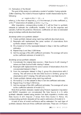
= exp( + ), = 1,2, … , (2.1)
where is the mean of response , is the intercept, is the coefficient, .

is the observation of variable Z, and = + .
ℎ

After imputation, corresponding models (2.1) will be fitted to synthetic
datasets to estimate the coefficients. Variable Y will be the response and
variable Z will be the predictor. Moreover, coefficients will also be estimated
using bootstrap methods described below.

Bootstrap within one synthetic dataset
1) Create synthetic dataset using matching methods described above.
2) Resample with replacement the same number of observations from
synthetic dataset created in Step 1.
3) Fit a model (2.1) to the resampled dataset in Step 2. Get the coefficient
estimates.
4) Repeat Step 2 and Step 3 200 times.
5) Get the average of the 200 coefficient estimates. The average will serve
as the coefficient estimate of model (2.1).

Bootstrap across synthetic datasets
1) Concatenate the original data sources – Data Source A with missing Z
values and Data Source B with missing Y values.
2) Resample with replacement the same number of observations from the
concatenated dataset in Step 1.
3) From the resampled dataset in Step 2, group the observations with Z
missing. This will serve as the new Data Source A. Similarly, group the
observations with Y missing. This will serve as the new Data Source B.
4) Create synthetic dataset using matching methods.
5) Fit model (2.1) to the dataset in Step 4. Get the coefficient estimates.
6) Repeat Step 2 to Step 5 200 times.
7) Get the average of the 200 coefficient estimates. The average will serve
as the coefficient estimate of model (2.1).
Note that synthetic datasets created using Poisson regression imputation
and MCMC imputation are concatenated file Data Source A ∪ B, while
synthetic datasets created using random hot deck imputation involve only
Data Source A with imputed Z values from Data Source B. Hence, the
corresponding synthetic datasets will be used in estimation of model (2.1).
A total of nine of model coefficients will be estimated. For each type of
synthetic dataset, there are three coefficient estimates. These are: (1) Poisson

14 | I S I W S C 2 0 1 9