Page 355 - Contributed Paper Session (CPS) - Volume 7

CPS2125 Dian Handayani et al.

See Berg and Chandra (2014) for further details of derivation of the closed
form of Mean Square Error (MSE) of and the estimates of MSE.

4. SEBP under Spatial Unit Level Lognormal Model
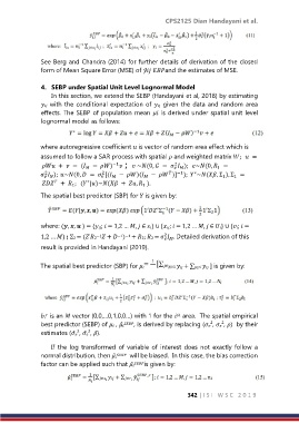
In this section, we extend the SEBP (Handayani et al, 2018) by estimating
with the conditional expectation of given the data and random area
effects. The SEBP of population mean is derived under spatial unit level
lognormal model as follows:

where autoregressive coefficient is vector of random area effect which is
assumed to follow a SAR process with spatial and weighted matrix ; =
2
−1
+ = ( − ) ; ~(0, = ); ~(0, =

1
2
2
−1
∗

); ~(0, = [( − )( − )] ); ~(, Σ ), Σ =
1

1
∗

+ ; ( |)~( + , ).
1
1
The spatial best predictor (SBP) for is given by:

where: (, , ) = {; = 1,2 … , ∈ } ∪ {; = 1,2 … , ∈ } ∪ {; =
1,2 … } ; Σ2 = ( 2 + ) + 2; 2 = σ . Detailed derivation of this
2
−1
′
−1 −1

result is provided in Handayani (2019).
The spatial best predictor (SBP) for + ∑∈ ] is given by:

is an vector (0,0,…0,1,0,0…) with 1 for the area. The spatial empirical

ℎ
2
2
, is derived by replacing ( , , ) by their
best predictor (SEBP) of ,
2
2
estimates ( , , ).
If the log transformed of variable of interest does not exactly follow a
will be biased. In this case, the bias correction
normal distribution, then
factor can be applied such that is given by:

342 | I S I W S C 2 0 1 9