Page 161 - Contributed Paper Session (CPS) - Volume 8

CPS2225 Retno Subekti et al.
about how and what method to ended up with posterior distribution. Idzorek
(2) proposed a guide to involve with Black Litterman in practice.
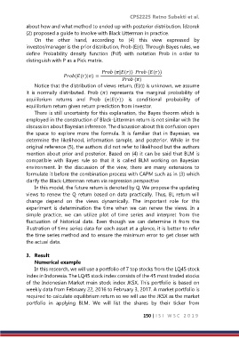
On the other hand, according to (4) this view expressed by
investor/manager is the prior distribution, Prob (E(r)). Through Bayes rules, we
define Probability density function (Pdf) with notation Prob in order to

distinguish with P as a Pick matrix.

(|()) (())
(()|) =
()
Notice that the distribution of views return, (E(r)) is unknown, we assume
it is normally distributed. Prob () represents the marginal probability of
equilibrium returns and Prob (|()) is conditional probability of
equilibrium return given return prediction from investor.
There is still uncertainty for this explanation, the Bayes theorm which is
employed in the construction of Black-Litterman return is not similar with the
discussion about Bayesian inference. The discussion about this confusion open
the space to explore more the formula. It is familiar that in Bayesian, we
determine the likelihood, information sample, and posterior. While in the
original reference (5), the authors did not refer to likelihood but the authors
mention about prior and posterior. Based on (4) it can be said that BLM is
compatible with Bayes rule so that it is called BLM working on Bayesian
environment. In the discussion of the view, there are many extensions to
formulate it before the combination process with CAPM such as in (3) which
clarify the Black-Litterman return via regression perspective
In this model, the future return is denoted by Q. We propose the updating
views to renew the Q return based on data practically. Thus, BL return will
change depend on the views dynamically. The important role for this
experiment is determination the time when we can renew the views. In a
simple practice, we can utilize plot of time series and interpret from the
fluctuation of historical data. Even though we can determine it from the
illustration of time series data for each asset at a glance, it is better to refer
the time series method and to ensure the minimum error to get closer with
the actual data.

3. Result
Numerical example
In this research, we will use a portfolio of 7 top stocks from the LQ45 stock
index in Indonesia. The LQ45 stock index consists of the 45 most traded stocks
of the Indonesian Market main stock index JKSX. This portfolio is based on
weekly data from February 22, 2016 to February 3, 2017. A market portfolio is
required to calculate equilibrium return so we will use the JKSX as the market
portfolio in applying BLM. We will list the shares by their ticker from

150 | I S I W S C 2 0 1 9