Page 164 - Contributed Paper Session (CPS) - Volume 8

CPS2225 Retno Subekti et al.

Portfolio Return 2

100.00%

50.00%

0.00%
May May May Jun Jun Jun Jun Jul 03, Jul 10, Jul 17,
-50.00% 15, 22, 29, 05, 12, 19, 26, 2017 2017 2017
2017 2017 2017 2017 2017 2017 2017
-100.00%

fMA2 fMA3 fMA4 fMA5 fMA6

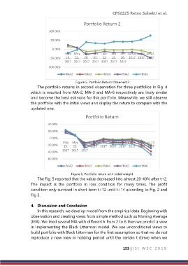
Figure 5. Portfolio Return Observed 2
The portfolio returns in second observation for three portfolios in Fig. 4
which is resulted from MA-2, MA-3 and MA-6 respectively are likely similar
and become the best estimate for this portfolio. Meanwhile, we still observe
the portfolio with the initial views and display the return to compare with the
updated one.

Portfolio Return

40.00%
20.00%

0.00%
May May May Jun 05,Jun 12,Jun 19,Jun 26, Jul 03, Jul 10, Jul 17,
-20.00%
15, 22, 29, 2017 2017 2017 2017 2017 2017 2017
2017 2017 2017
-40.00%
-60.00%
fMA2 fMA3 fMA4 fMA5 fMA6

Figure 6. Portfolio return with initial weight.
The Fig. 5 reported that the value decreased into almost 20-40% after t+2.
The impact is the portfolio in loss condition for many times. The profit
condition only survived in short term t+12 until t+14 according to Fig. 2 and
Fig 5.

4. Discussion and Conclusion
In this research, we develop model from the empirical data. Beginning with
observation and creating views from simple method such as Moving Average
(MA). We tried several MA with different k from 2 to 6 then we predict a view
in implementing the Black Litterman model. We use unconditional views to
build portfolio with Black Litterman for the first assumption so that we do not
reproduce a new view in holding period until the certain t (time) when we

153 | I S I W S C 2 0 1 9