Page 100 - Contributed Paper Session (CPS) - Volume 6

CPS1835 Lili Chen et al.
2. Methodology and Data
2.1 Methodology
This paper attempts to re-verify the EKC curve hypothesis, examines the
relationship between carbon emissions and economic development levels,
and reveals the role of economic levels in environmental pollution. The
expected result is in line with the inverted U-shaped relationship of the EKC
curve. With fast-growing economies and per capita income, the carbon
emissions will gradually increase, but when the per capita income reaches a
certain point, the carbon emissions will gradually decrease. After drawing on
and combining the methods of the predecessors and considering the
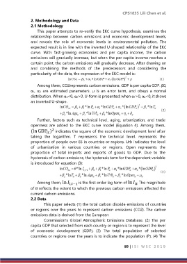
particularity of the data, the expression of the EKC model is:

Among them, CO2represents carbon emissions. GDP is per capita GDP. β0,
α1, α2 are estimated parameters. μ is an error term, and obeys a normal
distribution. When α1<0, α2>0, U-form is presented; when α1>0, α2<0, it shows
an inverted U-shape.

Further, factors such as technical level, aging, urbanization, and trade
openness are added to the EKC curve model (Equation 4). Among them,
2
(ln GDP ) indicates the square of the economic development level after

taking the logarithm. T represents the technical level. represents the
proportion of people over 65 in countries or regions. Urb indicates the level
of urbanization in various countries or regions. Open represents the
proportion of total imports and exports of goods to GDP. Due to the
hysteresis of carbon emissions, the hysteresis term for the dependent variable
is introduced for equation (3):

Among them, ln ,−1 is the first order lag term of ln The magnitude

of θ reflects the extent to which the previous carbon emissions affected the
current carbon emissions.
2.2 Data
This paper selects (1) the total carbon dioxide emissions of countries
or regions over the years to represent carbon emissions (CO2). The carbon
emissions data is derived from the European
Commission's Global Atmospheric Emissions Database. (2) The per
capita GDP that selected from each country or region is to represent the level
of economic development (GDP). (3) The total population of selected
countries or regions over the years is to indicate the population (P). (4) The

89 | I S I W S C 2 0 1 9