Page 73 - Contributed Paper Session (CPS) - Volume 6

CPS1810 Jin-Jian Hsieh et al.
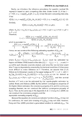
Nextly, we introduce the inference procedures for quantile residual life
regression based on semi-competing risks data. Under model (1), it has 1 −

)| ≥ , }. Under the semi-competing risks data,
= { ≥ + exp( |0 0
0

it has

[{ ≥ + exp( |0 0 |0
)} / ( )| ] = ( ≥ + exp(
) | ) (2)
0

Similarly,
[{ ≥ } / ( )| ] = ( ≥ | ), (3)

0

0

where ( ) = ( ) × |, ( | , ) = ( > | = ) × ( > | =

, = )

Therefore,

)} / ( )| ]
[{ ≥ + exp( |0

0
1 − = ,
[{ ≥ } / ( )| ]

0

which is equivalent to

)}
{ ≥ + exp( |0 { ≥ }
0

0

[ | ] − (1 − ) [ | ] = 0.

( ) ( )

Hence, we can construct the following estimating equation of |0 as:
{log( − ) ≥ } { ≥ }
0
( |0 ) = ∑ { |0 − (1 − ) 0 = 0} (4)

̂
̂
=1

̂
̂
̂
where ( ) = ( ) × ̂ |, ( | , ). ( ) could be estimated by

Kaplan and Meier (1958) based on the data {(, 1 − ), = 1, . . . , and =

} within each discrete covariate stratum, and since the non-terminal event

time may be dependently censored by the terminal event time D, it becomes
more difficult to make inference on . Therefore, we assume that (, )
follows an Archimedean copula on the upper wedge as ( > , > |) =
−1 { ( (|)) + ( (|))}, < . ̂ |, ( | , ) can be derived as

̂
̂ |, ( | , ) = ( > | = , = = ( ̂ | ( | )) , and the survival

′ ( ̂ ( | ))
|
function of and can be estimated by the copula-graphic estimator by
Lakhal, Rivest, and Abdous (2008). By the uniform convergence properties of
the Kaplan-Meier estimator, the consistency property of ,̂ and the continuous
mapping theorem, we can construct the uniform convergence property of
̂
(). Then, by the same way in the Appendix A, B, C in Jung et al. (2009), we

can construct the consistency property and the
asymptotic normality property of ̂ |0 .
Because the equation (4) contains an indicator function of |0 , it may not
be continuous. An exact zero-crossing of ( |0 ) may not exist. However,

Peng and Fine (2009) provided a generalized solution to estimate |0 . The
62 | I S I W S C 2 0 1 9