Page 83 - Invited Paper Session (IPS) - Volume 1

IPS61 Rituparna S. et al.
time series in the linear regression model, then the first time series can be
said to Granger-cause the second time series.
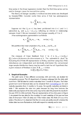
The theory of Granger causality in multivariate time series was developed
by Geweke(1982). Consider vector time series Z that has autoregressive
representation
∞
Z = ∑ +∈

−

=1

Suppose not that Z : × 1 has been partitioned into × 1 and × 1

subvectors , and , z′ = (x′ , y′ ), reflecting an interest in relationship

between X and Y. We are interested in the Granger causality of Y on X.
X has autoregressive representation as follows:
∞
= ∑ + , ( ) = ∑

−
1
=1

We partition the linear projection of on −1 −1 as

∞ ∞
= ∑ + ∑ + ( ) = ∑

−
2
−

=1 =1

The measure of linear feedback from to X is → = (|∑ |/
1
|∑ |) ℎ || ℎ . The estimation is done by
2
truncating the infinite AR representation at finite and then using OLS. If the
disturbances are independent and identically distributed, the conventional
large-sample distribution theory may be used to test the null hypothesis that
a given measure of feedback is zero. If → = 0, then
(|∑ |/|∑ )⟹ ().
2
̂
̂
1
2

3. Empirical Examples
The yield curve of two different economies, USA and India, are studied for
comparative purpose. The US department of treasury webpage lists the daily yield
curve from 1990 till date for certain maturities from 1 month to 30 years. The Indian
government bond historical data can be obtained from in.investing.com for each
maturity separately from 3 months to 15 years. The specific maturities are listed in
table 1. We separate the data into years because for long time horizons the
stationarity assumption of the time series may not be valid. We present the results for
the year 2015 for USA and India. They are representative of the other years. In Figure
1, we present the raw data for the countries. For each weekday of the year we have
data of dimension 11(for US data) and 17(for Indian data). We think of it as a time
series of functions. It is observed that the US curves are pretty smooth whereas the
Indian data has more fluctuations, both with respect to maturity and in time.

72 | I S I W S C 2 0 1 9