Page 213 - Special Topic Session (STS) - Volume 1

STS425 Nur I. et al.
model written as MSw(K)-AR(r). For r=1, the MSw(K)-AR(1) of equation
(1) can be written as

= (∅ 0 + ∅ 1 −1 ) + , = 1,2, … , (3)

The parameters estimation will estimate an unknown and optimal
number of regimes including their parameters simultaneously. However,
determining the optimal number of states representing any of the time
jumps is a hidden step in the MSwM estimation process. To do this, the
ordinary likelihood ratio tests may not be fulfilled, although it has a regular
2
condition for asymptotic distribution. Persio and Frigo (2016) have tried
to use an MLE to estimate the MSwM in a serial financial time modeling
by involving the external factors from its own data series for identifying
the hidden number of state.

2.2. Expectation Maximization and Average Run Length
The EM algorithm is a method for estimating a model having latent
parameters that are not given directly by the data. It works through two
stages, namely the Expectation stage and the Maximization stage,
iteratively until convergence to estimate parameters in the non-close form
likelihood function ((Dempster et. al, 1977) and (Susanto, 2018)).

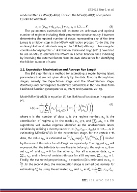
Model MSw(K)-AR(1) in equation (3) has likelihood function as in equation
(4).
1 1 2 (4)
() = ∏ ∑ ( ( ) (− ( ) ))
√2 2
2
=1 =1
where is the number of data, is the regime number, is the

contribution of regime in the model, ≥ 0, and ∑ = 1. EM

=1

algorithms will involve regimes identifier as the unobservable latent
variables by utilizing a dummy vector = ( , , … , ), = 1,2, … , , in

1

2
estimating MSw(K)-AR(r). In the expectation stage, for the certain -th
2
1
data, the value is estimated as ⁄ exp (− ⁄ ( ⁄ ) ) divided
2
by the sum of this value for all K regimes repeatedly. The biggest will

represent that the t-th data is more likely to belong to the regime , then

set =1 and = 0 for the other . For all number data, =

∑ , and in favor of certain -th data for all K regimes, ∑ = 1.
−1
=1

Finally, the estimated proportion in equation (4) is estimated as =

. In the second step, the maximization stage is carried out, namely for

2
2
2
estimating ̂ by using the estimated and as ̂ = 1 ∑ .
=1

202 | I S I W S C 2 0 1 9