Page 258 - Special Topic Session (STS) - Volume 1

STS426 Guillaume B.
The reason is that each power estimate is calculated from a sum of squared
standard normal variates.
2
The natural choice for a general optimal χ fit statistic is twice the negative
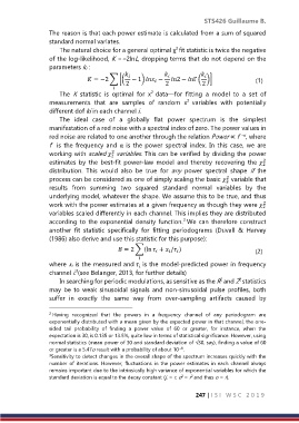
of the log-likelihood, K =−2lnL, dropping terms that do not depend on the
parameters ki :

= −2 ∑ [( 2 − 1) − 2 2 − Γ ( )] (1)

2

The K statistic is optimal for x data—for fitting a model to a set of
2
measurements that are samples of random x variables with potentially
2
different dof ki in each channel i.
The ideal case of a globally flat power spectrum is the simplest
manifestation of a red noise with a spectral index of zero. The power values in
red noise are related to one another through the relation Power ∝ f , where
−α
f is the frequency and α is the power spectral index. In this case, we are
2
working with scaled variables. This can be verified by dividing the power
2
2
estimates by the best-fit power-law model and thereby recovering the
2
distribution. This would also be true for any power spectral shape if the
process can be considered as one of simply scaling the basic variable that
2
2
results from summing two squared standard normal variables by the
underlying model, whatever the shape. We assume this to be true, and thus
work with the power estimates at a given frequency as though they were
2
2
variables scaled differently in each channel. This implies they are distributed
according to the exponential density function. We can therefore construct
2
another fit statistic specifically for fitting periodograms (Duvall & Harvey
(1986) also derive and use this statistic for this purpose):
= 2 ∑(ln + / ) (2)

where xi is the measured and is the model-predicted power in frequency

3
channel i. (see Belanger, 2013, for further details)
2
In searching for periodic modulations, as sensitive as the R and Z statistics
2
may be to weak sinusoidal signals and non-sinusoidal pulse profiles, both
suffer in exactly the same way from over-sampling artifacts caused by

2 Having recognized that the powers in a frequency channel of any periodogram are
exponentially distributed with a mean given by the expected power in that channel, the one-
sided tail probability of finding a power value of 60 or greater, for instance, when the
expectation is 30, is 0.135 or 13.5%, quite low in terms of statistical significance. However, using
normal statistics (mean power of 30 and standard deviation of √30, say), finding a value of 60
or greater is a 5.47o result with a probability of about 10 .
−8
3 Sensitivity to detect changes in the overall shape of the spectrum increases quickly with the
number of iterations. However, fluctuations in the power estimates in each channel always
remains important due to the intrinsically high variance of exponential variables for which the
standard deviation is equal to the decay constant (j. = r, o = r and thus o = r).
2
2

247 | I S I W S C 2 0 1 9