Page 29 - Special Topic Session (STS) - Volume 1
P. 29
STS346 A.H.M. Rahmatullah Imon


                                           − ̂  (−)   ∈
                                                   (−)
                                     ̂ (−) √(1 − ℎ   )
                                ∗
                                =                                                                  (7)

                                           − ̂  (−)

                                                            ∈
                                      ̂ (−) √(1 − ℎ (−) )
                                    {

                              ̂ (−)
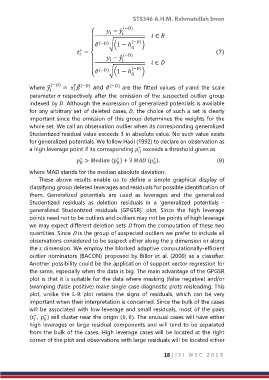
            where ̂  (−)  =      and ̂ (−)  are  the  fitted  values  of and  the  scale

            parameter  respectively after the omission of the suspected outlier group
            indexed by . Although the expression of generalized potentials is available
            for any arbitrary set of deleted cases, , the choice of such a set is clearly
            important since the omission of this group determines the weights for the
            whole set. We call an observation outlier when its corresponding generalized
            Studentized residual value exceeds 3 in absolute value. No such value exists
            for generalized potentials. We follow Hadi (1992) to declare an observation as
                                                      ∗
            a high leverage point if its corresponding   exceeds a threshold given as


                                                            ∗
                                              ∗
                                ∗
                               >  ( ) + 3  ( ).                                             (8)


            where MAD stands for the median absolute deviation.
                These  above  results  enable  us  to  define  a  simple  graphical  display  of
            classifying group deleted leverages and residuals for possible identification of
            them.  Generalized  potentials  are  used  as  leverages  and  the  generalized
            Studentized  residuals  as  deletion  residuals  in  a  ‘generalized  potentials  –
            generalized  Studentized  residuals  (GPGSR)’  plot.  Since  the  high  leverage
            points need not to be outliers and outliers may not be points of high leverage
            we may expect different deletion sets D from the computation of these two
            quantities. Since D is the group of suspected outliers we prefer to include all
            observations considered to be suspect either along the y dimension or along
            the  dimension. We employ the blocked adaptive computationally-efficient
            outlier nominators (BACON) proposed by Billor et al. (2000)  as a classifier.
            Another possibility could be the application of support vector regression for
            the same, especially when the data is big. The main advantage of the GPGSR
            plot is that it is suitable for the data where masking (false negative) and/or
            swamping (false positive) make single case diagnostic plots misleading. This
            plot,  unlike  the  L-R  plot  retains  the  signs  of  residuals,  which  can  be  very
            important when their interpretation is concerned. Since the bulk of the cases
            will be associated with low leverage and small residuals, most of the pairs
              ∗
            ( ,  ) will cluster near the origin (0, 0). The unusual cases will have either
                  ∗


            high leverages or large residual components and will tend to be separated
            from the bulk of the cases. High leverage cases will be located at the right
            corner of the plot and observations with large residuals will be located either
                                                                18 | I S I   W S C   2 0 1 9

