Page 31 - Special Topic Session (STS) - Volume 1

STS346 A.H.M. Rahmatullah Imon
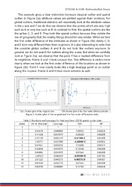
This example gives a clear distinction between classical outlier and spatial
outlier. In Figure 2(a) attribute values are plotted against their locations. For
global outliers, traditional statistics will essentially look at the attribute values
in the y axis and if we do that we observe that the points which are very high
such as A or very low such as B. In contrast to that, the spatial outliers are like
the spikes C, D, and E. They look like spatial outliers because they violate the
law of geography that the nearby things should be very similar. When we take
the first order difference of the attributes as shown in Figure 2(b) clearly C, D,
and E look very different than their neighbors. It is also interesting to note that
the possible global outliers A and B do not look like outliers anymore. In
general, we do not search for outliers along the x-axis. But when we carefully
look at Figure 2(a), we observe that the point F has a marked difference from
its neighbors. Points G and H look unusual too. This difference is visible more
clearly when we look at the first order difference of the locations as shown in
Figure 2(b). Point F now clearly looks like a high leverage point or an outlier
along the x-space. Points G and H look more extreme as well.

Figure 2: Scatter plot of the original and the first order differenced data.

Table 2: Residuals and leverages for Hadi and Imon (2018) spatial outlier data
Index Del St. Residual Leverage GSR GP
1 * * * *
2 0.45678 0.040885 1.09925 0.06658
3 0.11424 0.051079 0.20420 0.06290
4 2.15139 0.035779 5.31765 C 0.03590
5 -1.69711 0.037989 -4.20445 C 0.03835
6 0.47421 0.035612 1.13209 0.04571
7 0.32834 0.051079 0.72348 0.06290
8 0.06085 0.051079 0.07645 0.06290
9 -2.41622 0.045639 -6.03394 D 0.05185
10 2.61223 0.041275 6.49375 D 0.04367
11 0.07639 0.035779 0.07645 0.03590
12 0.89298 0.040885 0.13783 0.06658

20 | I S I W S C 2 0 1 9