Page 345 - Special Topic Session (STS) - Volume 3

STS550 Pierre Guérin et al.
to implement and offers a great deal of flexibility in modelling time variation
since we do not restrict the regime changes in the cross-sectional dimension
to be governed by a single or a limited number of Markov chains.

2. Markov-Switching Three-Pass Regression Filter
One key reason for the absence of a significant literature on large-scale
Markov-switching factor models relates to the computational challenges
associated with the estimation of such models. We present here the Markov-
switching three-pass regression filter, which circumvents these difficulties.
Our setting is similar to that in Kelly and Pruitt (2015), who introduced the
linear 3PRF, but the key novelty is that we include time variation in the model
parameters via Markov processes. Specifically, we have the following model:
= ( ) + ( ) −1 + , = 1, … , , (1)

0

= ( ) + ( ) + , = 1, … , (2)

0,

= ∅ ( ) + ∅ ( ) + ∅ ( ) + , = 1, … , , (3)
,

,

,

where is the scalar target variable of interest for forecasting; = ( , ...,

1
)' is a × 1 vector of unobservable factors, with associated slope

coefficients ( ); = 1, … , , are so-called proxy variables driven by

,

the same factors as , , with variable specific loadings ( ); =

1, … , , are variables driven by the factors but also by the

(unobservable) factors in the vector , with associated variable specific

loadings ∅ ( ) and ∅ ( ) respectively; ( ) , ( ), ∅ ( )
,
,
,
0,

0
are intercepts. As anticipated, the coefficients in (1) to (3) are time-varying
and driven by variable specific and independent across variables M-state
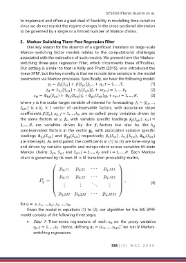
Markov chains: , and = 1, …, and = 1, … , . Each Markov

chain is governed by its own × transition probability matrix,

(4)

for = , , … , , , … , .

1

1
Given the model in equations (1) to (3), our algorithm for the MS-3PRF
model consists of the following three steps:
• Step 1: Time-series regressions of each on the proxy variables
, = 1, … , . Hence, defining = ( , … , )′, we run Markov-
1

switching regressions
334 | I S I W S C 2 0 1 9