Page 380 - Special Topic Session (STS) - Volume 4

STS2319 Lakshman N. R. et al.
through a curve fitting from the fused data points. Harvest Index requires
spatially variable weather data and/or multiple-season data to capture the
impact of climatic conditions. In this study, we only have crop cutting data for
one growing season. Also, given the relatively small area of Thai Binh, there
may not be significant variation in climatic variables across the province. Thus,
we primarily focus on approximating AGB for yield estimation, under the
assumption that all rice fields in the province share the same harvest index for
the current growing season.
To overcome the large gaps and the noises of both positives and
negatives in our time series data, we use a simple quadratic curve fitting
method to derive peak vegetation indexes of the second growing season. The
quadratic curve is centered at DOY 250, which was determined by visually
inspecting many time series of crop pixels distributed over the study area. To
reduce the impact of noises in the time series to our peak estimation, we
calculate the standard deviation of the fitted curve and remove vegetation
index values beyond three standard deviations from the mean. Then a new
curve is fitted to the remaining vegetation index values. This procedure is
repeated iteratively until all the vegetation index values for the curve fitting
are within the confidence interval of the curve fitting. The derived peak
vegetation index values of the pixels of all the representative field subplots are
then regressed against the crop cutting yield data. We use NDVI, EVI, and GCVI
peak values respectively to derive univariate linear regression models.

3. Results
A. Landsat–MODIS Fusion
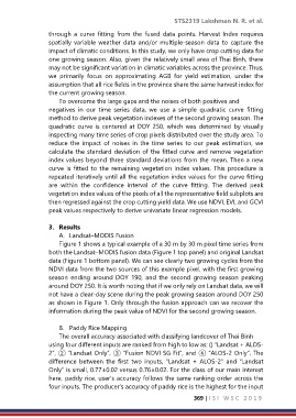
Figure 1 shows a typical example of a 30 m by 30 m pixel time series from
both the Landsat–MODIS fusion data (Figure 1 top panel) and original Landsat
data (Figure 1 bottom panel). We can see clearly two growing cycles from the
NDVI data from the two sources of this example pixel, with the first growing
season ending around DOY 190, and the second growing season peaking
around DOY 250. It is worth noting that if we only rely on Landsat data, we will
not have a clear-day scene during the peak growing season around DOY 250
as shown in Figure 1. Only through the fusion approach can we recover the
information during the peak value of NDVI for the second growing season.

B. Paddy Rice Mapping
The overall accuracy associated with classifying landcover of Thai Binh
using four different inputs are ranked from high to low as: () “Landsat + ALOS-
2”, ② “Landsat Only”, ③ “Fusion NDVI SG Fit”, and ④ “ALOS-2 Only”. The
difference between the first two inputs, “Landsat + ALOS-2” and “Landsat
Only” is small, 0.77±0.02 versus 0.76±0.02. For the class of our main interest
here, paddy rice, user’s accuracy follows the same ranking order across the
four inputs. The producer’s accuracy of paddy rice is the highest for the input

369 | I S I W S C 2 0 1 9