Page 71 - Special Topic Session (STS) - Volume 4

STS563 Patrick Graham et al.
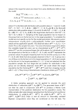
values in the target-list union are drawn from some distribution G(θ) we have
the model

where if is the Bernoulli distribution with possible values (1, 1) and (0, 1) with
Pr( = (1, 1)| = (1, 1), X, λ) = λ(X);if = (1, 0), (1,0)(λ, X) is the Bernoulli
̃
distribution with possible values (1, 0) and (0, 0) with Pr( = (1, 0)| = (1, 0), X,
̃
λ) = λ(X); if = (0, 1), (0,1)(λ, X) is the degenerate distribution with Pr( = (0,
̃
1)| = (0, 1), X, λ) = 1. Sampling of the target population has no impact on
the group that is on the list but not in the target population. To complete the
model we must specify a prior for the model parameters. We assume a priori
independence so ( , , ) = ( )()(). Further prior specification

̃
̃
details will be application specific. The observed data is = ( , ; ∶ ≠

(0,0)0. This is the sample-list union. The extra information required to obtain
the complete target-list union can be characterised as = ( , )
where are the unobserved target-list cell locations for individuals not in

̃
the sample but on the list (i.e. in the ( = (0, 1) cell), and represents the
covariate values for people missed by both the list and the survey (i.e in the

= (0, 0) cell). Note that since people observed in the = (0, 1) group are a
̃
̃
mix of those on the list but not in the target population ( =(0,1)) and people
on the list and in the target population ( = (1, 1)) but not selected into the
population sample, the true target-list cell location for individuals in this
group are not directly observed. Given we could obtain the target
population by first forming = ( , ) and then dropping records
with = (0, 1). The primary inferential task is therefore to obtain ( | ):
( , | ) = ∫ ( | , , ) ( , | )

= ∫ ( , , | )

A Gibbs sampling approach can be applied to simulate the joint
distribution of unknowns ( , , | ). The generated draws of

can then be used in conjunction with to produce a Monte Carlo
representation of the posterior distribution for the population counts. The
Gibbs sampler alternates between sampling from the following full conditional

distributions: (i) (|∅, , , ); (ii) (∅|, , , ); (iii)

( , | , ∅, ). Steps (i) and (ii) amount to reasonably standard

Bayesian computations since they are conditional on the full data. The

60 | I S I W S C 2 0 1 9