Page 22 - Contributed Paper Session (CPS) - Volume 1

CPS653 Chang-Yun L.
that Σ is a biased estimator of Σ (Kenward and Roger, 1997), and Vare
̃
̃
̂
commonly used for hypothesis tests in the regression methods.
For SPDS and BDS designs, the full second-order model is inestimable due
to insufficient degrees of freedom. Hence, the process for model selections
must be implemented. Two regression methods, MSR and FSR, have been
proposed in the literature for performing model selections for SPDS and BDS
designs. The two methods have the following limitations: (i) the active effects
cannot be estimated if the number of them is greater than the rank of the
model matrix and (ii) ̂ = 0 may be obtained by using the REML method. To

circumvent these problems, we propose a Bayesian variable selection method
as described in the next section.

3. Stochastic search variable selection
Let = ( , , , , ) denote the vector of the model parameters,
′
′
′
′

where = ( ,· · · , , ,· · · , −1, , ,· · · , )′ . By the Baye’s
11
1
12

Theorem (see DeGroot, 1970, p28, and Robinson et al., 2012), the joint
posterior density of the model parameters is proportional to the product of
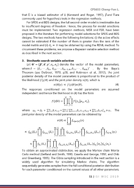
the likelihood (y|Θ) and the joint prior density π(Θ), which is

(|) ∝ (|)(). (4)

The responses conditioned on the model parameters are assumed
independent and hence the likelihood in (4) has the form

(y|Θ) = ∏ ∏ ( | , ),

−1 =1

where µ = + ∑ + ∑ −1 ∑ + ∑ 2 + . The
=1
=1
,

,
=1

=+1
, ,
0
joint prior density of the model parameters can be obtained by

(Θ) ∝ ∏ |[] ()
∈Θ

−1
∝ ( ) ∏ ( ) ∏ ∏ ( ) ∏ ( ) ∏ ( )
0 0 | | | |
=1 =1 =+1 =1 =1

−1
× ∏ ( ) ∏ ∏ ( ) ∏ ( ) ( ) ( ).
| , |
=1 −1 =+1 =1
To obtain an approximated distribution, we apply the Markov chain Monte
Carlo method (Gelfand and Smith, 1990, Casella and George, 1992, and Chib
and Greenberg, 1995). The Gibbs sampling introduced in the next section is a
widely used algorithm for simulating Markov chains. The algorithm
sequentially generates samples from the full conditional posterior distribution
for each parameter conditioned on the current values of all other parameters.
11 | I S I W S C 2 0 1 9